V2: Convergence Pooling

Vignette 2 of 8 · Compare to Algorithmic convergence and inference pooling by Gerko Vink and Stef van Buuren

62% exact · 16 match · 5 info · 5 visual · 0 skipped

This walkthrough mirrors the official R **mice** tutorials in Python. Deterministic tables and formulas are checked against the R reference; stochastic imputations and plots are labelled when they may differ.

What PyMICE does differently from R

Default randomness uses NumPy (rng="numpy"), so imputed values may differ from R unless you set rng="r".
Categorical factors are often shown as numeric codes in console output.
Diagnostic figures use matplotlib instead of lattice (same intent, different styling).
See REPRODUCIBILITY.md for exact replication options.

Parity details (maintainers)

Expected to match exactly

These numbered steps are checked against reference/02_convergence_and_pooling/vignette_extracted.R:

Step 2 — default and modified pred matrices; maxit=0 initializer matrix
Step 4 — imp$meth on nhanes and nhanes2; summary(nhanes2) factor layout; methods(mice) listing (static reference text)
Step 7 — class(fit) and ls(fit) names; print(fit) mira coefficients (exact=True); summary(fit$analyses[[2]]) on imp3 (atol=0.15)
Step 8 — pooled summary(pool.fit) (exact=True; session R stream; goldens refreshed 2026-07-05)

Expected to differ (RNG / rendering)

Step 1 — mice(nhanes, m=3) setup; no R console output to compare.
Step 3 — plot(imp) matplotlib trace plots; diagnostic shape matches, not pixel-identical to lattice.
Step 4 — str(nhanes2) (factor labels vs numeric codes); plot(imp) on nhanes2.
Step 5 — extended trace via continue_imputation(imp3, maxit=35) (R mice.mids warm start).
Step 6 — stripplot() matplotlib diagnostics; observed/imputed colours differ from lattice.

Partial (quickpred)

Step 2 — quickpred(nhanes, mincor=.3) predictor matrix matches R golden layout.

Introduction

This is the second vignette in a series of six.

The aim of this vignette is to enhance your understanding of multiple imputation, in general. You will learn how to pool the results of analyses performed on multiply-imputed data, how to approach different types of data and how to avoid the pitfalls researchers may fall into. The main objective is to increase your knowledge and understanding on applications of multiple imputation.

No previous experience with R is required. Again, we start by loading (with require()) the necessary packages and fixing the random seed to allow for our outcomes to be replicable.

require(mice) require(lattice) set.seed(123)

1. Vary number of imputations

Step parity: ✅ MATCH (0 exact, 2 info, 0 visual, 0 skipped, 0 mismatch of 2 blocks)

Note: Package load step; no R console output to compare.

Python (PyMICE)

import numpy as np
from pymice import mice, pool, with_mids, summary_pool, quickpred, complete
from pymice.diagnostics.plots import plot_mids, plot_stripplot
from lib.data import load_nhanes, load_nhanes2
from lib.viz import save_figure
from lib.r_style import (
    format_meth_r,
    format_pool_print_r,
    format_pool_tibble_r,
    format_predictor_matrix,
    format_summary_r,
    format_mira_print_r,
    format_lm_summary_r,
    format_pool_v02_r
)

Console Output

(setup — no console output)

R (Reference)

require(mice)
require(lattice)
set.seed(123)

import numpy as np
from pymice import mice, pool, with_mids, summary_pool, quickpred, complete
from pymice.diagnostics.plots import plot_mids, plot_stripplot
from lib.data import load_nhanes, load_nhanes2
from lib.viz import save_figure
from lib.r_style import (
    format_meth_r,
    format_pool_print_r,
    format_pool_tibble_r,
    format_predictor_matrix,
    format_summary_r,
    format_mira_print_r,
    format_lm_summary_r,
    format_pool_v02_r
)

Console Output

(setup — no console output)

require(mice)
require(lattice)
set.seed(123)

The number of imputed data sets can be specified by the m = ... argument. For example, to create just three imputed data sets, specify

Note: Step creates imp object; R vignette prints no console output here.

Python (PyMICE)

imp_m3 = mice(data, column_names=names, m=3, maxit=5, seed=123, print_flag=False)

Console Output

(m = 3 imputation complete — no printed output in R vignette)

R (Reference)

imp <- mice(nhanes, m = 3, print=F)

imp_m3 = mice(data, column_names=names, m=3, maxit=5, seed=123, print_flag=False)

Console Output

(m = 3 imputation complete — no printed output in R vignette)

imp <- mice(nhanes, m = 3, print=F)

2. Edit predictor matrix

Step parity: ✅ MATCH (4 exact, 1 info, 0 visual, 0 skipped, 0 mismatch of 5 blocks)

The predictor matrix is a square matrix that specifies the variables that are used to impute each incomplete variable. Let us have a look at the predictor matrix that was used

Python (PyMICE)

print(format_predictor_matrix(names, imp_m3.predictor_matrix))

Console Output

    age bmi hyp chl
age     0   1   1   1
bmi     1   0   1   1
hyp     1   1   0   1
chl     1   1   1   0

R (Reference)

imp$pred

R Console Output

    age bmi hyp chl
age   0   1   1   1
bmi   1   0   1   1
hyp   1   1   0   1
chl   1   1   1   0

print(format_predictor_matrix(names, imp_m3.predictor_matrix))

Console Output

    age bmi hyp chl
age     0   1   1   1
bmi     1   0   1   1
hyp     1   1   0   1
chl     1   1   1   0

imp$pred

R Console Output

    age bmi hyp chl
age   0   1   1   1
bmi   1   0   1   1
hyp   1   1   0   1
chl   1   1   1   0

Each variable in the data has a row and a column in the predictor matrix. A value 1 indicates that the column variable was used to impute the row variable. For example, the 1 at entry [bmi, age] indicates that variable age was used to impute the incomplete variable bmi. Note that the diagonal is zero because a variable is not allowed to impute itself. The row of age contains all zeros because there were no missing values in age. mice gives you complete control over the predictor matrix, enabling you to choose your own predictor relations. This can be very useful, for example, when you have many variables or when you have clear ideas or prior knowledge about relations in the data at hand. You can use mice() to give you the initial predictor matrix, and change it afterwards, without running the algorithm. This can be done by typing

Python (PyMICE)

print(format_predictor_matrix(names, ini0.predictor_matrix))

Console Output

    age bmi hyp chl
age     0   1   1   1
bmi     1   0   1   1
hyp     1   1   0   1
chl     1   1   1   0

R (Reference)

ini <- mice(nhanes, maxit=0, print=F)
pred <- ini$pred
pred

R Console Output

    age bmi hyp chl
age   0   1   1   1
bmi   1   0   1   1
hyp   1   1   0   1
chl   1   1   1   0

print(format_predictor_matrix(names, ini0.predictor_matrix))

Console Output

    age bmi hyp chl
age     0   1   1   1
bmi     1   0   1   1
hyp     1   1   0   1
chl     1   1   1   0

ini <- mice(nhanes, maxit=0, print=F)
pred <- ini$pred
pred

R Console Output

    age bmi hyp chl
age   0   1   1   1
bmi   1   0   1   1
hyp   1   1   0   1
chl   1   1   1   0

The object pred contains the predictor matrix from an initial run of mice with zero iterations, specified by maxit = 0. Altering the predictor matrix and returning it to the mice algorithm is very simple. For example, the following code removes the variable hyp from the set of predictors, but still leaves it to be predicted by the other variables.

Python (PyMICE)

pred[:, names.index('hyp')] = 0
print(format_predictor_matrix(names, pred))

Console Output

    age bmi hyp chl
age     0   1   0   1
bmi     1   0   0   1
hyp     1   1   0   1
chl     1   1   0   0

R (Reference)

pred[ ,"hyp"] <- 0
pred

R Console Output

    age bmi hyp chl
age   0   1   0   1
bmi   1   0   0   1
hyp   1   1   0   1
chl   1   1   0   0

pred[:, names.index('hyp')] = 0
print(format_predictor_matrix(names, pred))

Console Output

    age bmi hyp chl
age     0   1   0   1
bmi     1   0   0   1
hyp     1   1   0   1
chl     1   1   0   0

pred[ ,"hyp"] <- 0
pred

R Console Output

    age bmi hyp chl
age   0   1   0   1
bmi   1   0   0   1
hyp   1   1   0   1
chl   1   1   0   0

Use your new predictor matrix in mice() as follows

Note: R vignette shows code only; no console output to compare.

Python (PyMICE)

mice(data, column_names=names, predictor_matrix=pred_mod, seed=123, print_flag=False)

Console Output

(imputation with custom predictor matrix — no printed output)

R (Reference)

imp <- mice(nhanes, pred=pred, print=F)

mice(data, column_names=names, predictor_matrix=pred_mod, seed=123, print_flag=False)

Console Output

(imputation with custom predictor matrix — no printed output)

imp <- mice(nhanes, pred=pred, print=F)

There is a special function called quickpred() for a quick selection procedure of predictors, which can be handy for datasets containing many variables. See ?quickpred for more info. Selecting predictors according to data relations with a minimum correlation of ρ = .30 can be done by

Python (PyMICE)

print(format_predictor_matrix(names, pred_quick))

Console Output

    age bmi hyp chl
age     0   0   0   0
bmi     1   0   0   1
hyp     1   0   0   1
chl     1   1   1   0

R (Reference)

ini <- mice(nhanes, pred=quickpred(nhanes, mincor=.3), print=F)
ini$pred

R Console Output

    age bmi hyp chl
age   0   0   0   0
bmi   1   0   0   1
hyp   1   0   0   1
chl   1   1   1   0

print(format_predictor_matrix(names, pred_quick))

Console Output

    age bmi hyp chl
age     0   0   0   0
bmi     1   0   0   1
hyp     1   0   0   1
chl     1   1   1   0

ini <- mice(nhanes, pred=quickpred(nhanes, mincor=.3), print=F)
ini$pred

R Console Output

    age bmi hyp chl
age   0   0   0   0
bmi   1   0   0   1
hyp   1   0   0   1
chl   1   1   1   0

For large predictor matrices, it can be useful to export them to Microsoft Excel for easier configuration (e.g. see the xlsx package for easy exporting and importing of Excel files).

3. Convergence trace plot

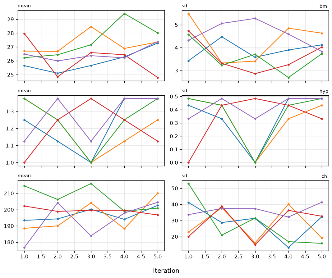
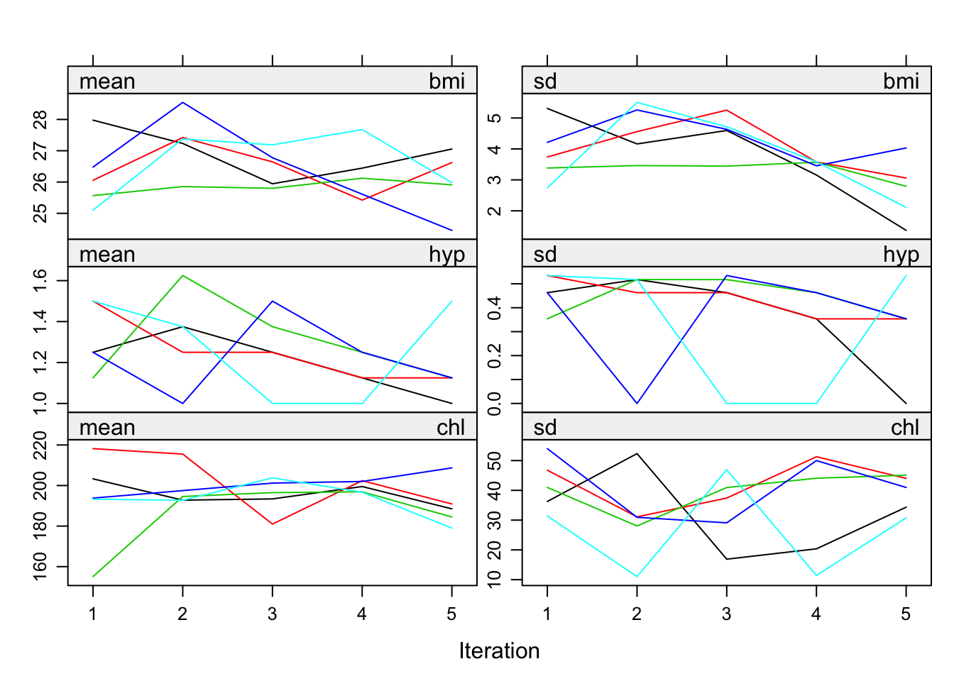
Step parity: ✅ MATCH (0 exact, 1 info, 1 visual, 0 skipped, 0 mismatch of 2 blocks)

The mice() function implements an iterative Markov Chain Monte Carlo type of algorithm. Let us have a look at the trace lines generated by the algorithm to study convergence:

Note: Matplotlib trace plot (mean imputations per iteration).

Python (PyMICE)

fig = plot_mids(imp_conv, variables=['bmi', 'hyp', 'chl'])
save_figure(fig, ASSETS, 'v02_plot_mids.png')

Console Output

(plot below)

R (Reference)

imp <- mice(nhanes, print=F)
plot(imp)

fig = plot_mids(imp_conv, variables=['bmi', 'hyp', 'chl'])
save_figure(fig, ASSETS, 'v02_plot_mids.png')

Console Output

(plot below)

imp <- mice(nhanes, print=F)
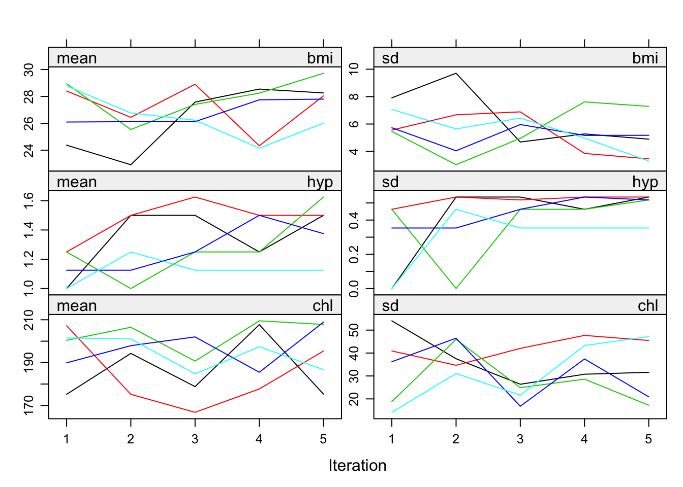
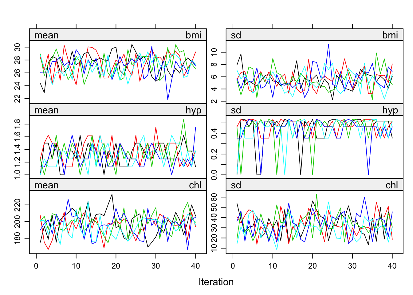
plot(imp)

The plot shows the mean (left) and standard deviation (right) of the imputed values only. In general, we would like the streams to intermingle and be free of any trends at the later iterations.

The algorithm uses random sampling, and therefore, the results will be (perhaps slightly) different if we repeat the imputations with different seeds. In order to get exactly the same result, use the seed argument

Note: Seed argument demonstration; no console output in R vignette.

Python (PyMICE)

imp_conv = mice(data, column_names=names, m=5, maxit=5, seed=123, print_flag=False)

Console Output

(reproducible imputation — no printed output)

R (Reference)

imp <- mice(nhanes, seed=123, print=F)

imp_conv = mice(data, column_names=names, m=5, maxit=5, seed=123, print_flag=False)

Console Output

(reproducible imputation — no printed output)

imp <- mice(nhanes, seed=123, print=F)

where 123 is some arbitrary number that you can choose yourself. Rerunning this command will always yields the same imputed values.

Python (PyMICE)

3. Convergence trace plot — v02_trace_nhanes.png

R (Reference)

4. Change imputation method

Step parity: ✅ MATCH (7 exact, 1 info, 1 visual, 0 skipped, 0 mismatch of 9 blocks)

For each column, the algorithm requires a specification of the imputation method. To see which method was used by default:

Python (PyMICE)

print(format_meth_r(names, imp_conv_seed.method, style='nhanes'))

Console Output

  age   bmi   hyp   chl
   "" "pmm" "pmm" "pmm"

R (Reference)

imp$meth

R Console Output

  age   bmi   hyp   chl
   "" "pmm" "pmm" "pmm"

print(format_meth_r(names, imp_conv_seed.method, style='nhanes'))

Console Output

  age   bmi   hyp   chl
   "" "pmm" "pmm" "pmm"

imp$meth

R Console Output

  age   bmi   hyp   chl
   "" "pmm" "pmm" "pmm"

The variable age is complete and therefore not imputed, denoted by the "" empty string. The other variables have method pmm, which stands for predictive mean matching, the default in mice for numerical and integer data. In reality, the data are better described a as mix of numerical and categorical data. Let us take a look at the nhanes2 data frame

Python (PyMICE)

print(format_summary_nhanes2_r(data2, names2))

Console Output

    age          bmi          hyp          chl
 20-39:12   Min.   :20.40   no  :13   Min.   :113.0
 40-59: 7   1st Qu.:22.65   yes : 4   1st Qu.:185.0
 60-99: 6   Median :26.75   NA's: 8   Median :187.0
            Mean   :26.56             Mean   :191.4
            3rd Qu.:28.93             3rd Qu.:212.0
            Max.   :35.30             Max.   :284.0
            NA's   : 9                 NA's   :10

R (Reference)

summary(nhanes2)

R Console Output

    age          bmi          hyp          chl
 20-39:12   Min.   :20.40   no  :13   Min.   :113.0
 40-59: 7   1st Qu.:22.65   yes : 4   1st Qu.:185.0
 60-99: 6   Median :26.75   NA's: 8   Median :187.0
            Mean   :26.56             Mean   :191.4
            3rd Qu.:28.93             3rd Qu.:212.0
            Max.   :35.30             Max.   :284.0
            NA's   :9                 NA's   :10

print(format_summary_nhanes2_r(data2, names2))

Console Output

    age          bmi          hyp          chl
 20-39:12   Min.   :20.40   no  :13   Min.   :113.0
 40-59: 7   1st Qu.:22.65   yes : 4   1st Qu.:185.0
 60-99: 6   Median :26.75   NA's: 8   Median :187.0
            Mean   :26.56             Mean   :191.4
            3rd Qu.:28.93             3rd Qu.:212.0
            Max.   :35.30             Max.   :284.0
            NA's   : 9                 NA's   :10

summary(nhanes2)

R Console Output

    age          bmi          hyp          chl
 20-39:12   Min.   :20.40   no  :13   Min.   :113.0
 40-59: 7   1st Qu.:22.65   yes : 4   1st Qu.:185.0
 60-99: 6   Median :26.75   NA's: 8   Median :187.0
            Mean   :26.56             Mean   :191.4
            3rd Qu.:28.93             3rd Qu.:212.0
            Max.   :35.30             Max.   :284.0
            NA's   :9                 NA's   :10

and the structure of the data frame

Python (PyMICE)

# str() layout — R factor labels vs numeric codes in PyMICE

Console Output

'data.frame':    25 obs. of  4 variables:
 $ age: Factor w/ 3 levels "20-39","40-59",..: 1 2 1 3 1 3 1 1 2 2 ...
 $ bmi: num  NA 22.7 NA NA 20.4 NA 22.5 30.1 22 NA ...
 $ hyp: Factor w/ 2 levels "no","yes": NA 1 1 NA 1 NA 1 1 1 NA ...
 $ chl: num  NA 187 187 NA 113 184 118 187 238 NA ...

R (Reference)

str(nhanes2)

R Console Output

'data.frame':    25 obs. of  4 variables:
 $ age: Factor w/ 3 levels "20-39","40-59",..: 1 2 1 3 1 3 1 1 2 2 ...
 $ bmi: num  NA 22.7 NA NA 20.4 NA 22.5 30.1 22 NA ...
 $ hyp: Factor w/ 2 levels "no","yes": NA 1 1 NA 1 NA 1 1 1 NA ...
 $ chl: num  NA 187 187 NA 113 184 118 187 238 NA ...

# str() layout — R factor labels vs numeric codes in PyMICE

Console Output

'data.frame':    25 obs. of  4 variables:
 $ age: Factor w/ 3 levels "20-39","40-59",..: 1 2 1 3 1 3 1 1 2 2 ...
 $ bmi: num  NA 22.7 NA NA 20.4 NA 22.5 30.1 22 NA ...
 $ hyp: Factor w/ 2 levels "no","yes": NA 1 1 NA 1 NA 1 1 1 NA ...
 $ chl: num  NA 187 187 NA 113 184 118 187 238 NA ...

str(nhanes2)

R Console Output

'data.frame':    25 obs. of  4 variables:
 $ age: Factor w/ 3 levels "20-39","40-59",..: 1 2 1 3 1 3 1 1 2 2 ...
 $ bmi: num  NA 22.7 NA NA 20.4 NA 22.5 30.1 22 NA ...
 $ hyp: Factor w/ 2 levels "no","yes": NA 1 1 NA 1 NA 1 1 1 NA ...
 $ chl: num  NA 187 187 NA 113 184 118 187 238 NA ...

Variable age consists of 3 age categories, while variable hyp is binary. The mice() function takes these properties automatically into account. Impute the nhanes2 dataset

Python (PyMICE)

print(format_meth_r(names2, imp2.method))

Console Output

     age      bmi      hyp      chl
      ""    "pmm"    "logreg"    "pmm"

R (Reference)

imp <- mice(nhanes2, print=F)
imp$meth

R Console Output

     age      bmi      hyp      chl
      ""    "pmm" "logreg"    "pmm"

print(format_meth_r(names2, imp2.method))

Console Output

     age      bmi      hyp      chl
      ""    "pmm"    "logreg"    "pmm"

imp <- mice(nhanes2, print=F)
imp$meth

R Console Output

     age      bmi      hyp      chl
      ""    "pmm" "logreg"    "pmm"

Notice that mice has set the imputation method for variable hyp to logreg, which implements multiple imputation by logistic regression.

An up-to-date overview of the methods in mice can be found by

Python (PyMICE)

# static R methods() listing (reference)

Console Output

 [1] mice.impute.2l.bin       mice.impute.2l.lmer     
 [3] mice.impute.2l.norm      mice.impute.2l.pan      
 [5] mice.impute.2lonly.mean  mice.impute.2lonly.norm 
 [7] mice.impute.2lonly.pmm   mice.impute.cart        
 [9] mice.impute.jomoImpute   mice.impute.lda         
[11] mice.impute.logreg       mice.impute.logreg.boot 
[13] mice.impute.mean         mice.impute.midastouch  
[15] mice.impute.norm         mice.impute.norm.boot   
[17] mice.impute.norm.nob     mice.impute.norm.predict
[19] mice.impute.panImpute    mice.impute.passive     
[21] mice.impute.pmm          mice.impute.polr        
[23] mice.impute.polyreg      mice.impute.quadratic   
[25] mice.impute.rf           mice.impute.ri          
[27] mice.impute.sample       mice.mids               
[29] mice.theme              
see '?methods' for accessing help and source code

R (Reference)

methods(mice)

R Console Output

 [1] mice.impute.2l.bin       mice.impute.2l.lmer     
 [3] mice.impute.2l.norm      mice.impute.2l.pan      
 [5] mice.impute.2lonly.mean  mice.impute.2lonly.norm 
 [7] mice.impute.2lonly.pmm   mice.impute.cart        
 [9] mice.impute.jomoImpute   mice.impute.lda         
[11] mice.impute.logreg       mice.impute.logreg.boot 
[13] mice.impute.mean         mice.impute.midastouch  
[15] mice.impute.norm         mice.impute.norm.boot   
[17] mice.impute.norm.nob     mice.impute.norm.predict
[19] mice.impute.panImpute    mice.impute.passive     
[21] mice.impute.pmm          mice.impute.polr        
[23] mice.impute.polyreg      mice.impute.quadratic   
[25] mice.impute.rf           mice.impute.ri          
[27] mice.impute.sample       mice.mids               
[29] mice.theme              
see '?methods' for accessing help and source code

# static R methods() listing (reference)

Console Output

 [1] mice.impute.2l.bin       mice.impute.2l.lmer     
 [3] mice.impute.2l.norm      mice.impute.2l.pan      
 [5] mice.impute.2lonly.mean  mice.impute.2lonly.norm 
 [7] mice.impute.2lonly.pmm   mice.impute.cart        
 [9] mice.impute.jomoImpute   mice.impute.lda         
[11] mice.impute.logreg       mice.impute.logreg.boot 
[13] mice.impute.mean         mice.impute.midastouch  
[15] mice.impute.norm         mice.impute.norm.boot   
[17] mice.impute.norm.nob     mice.impute.norm.predict
[19] mice.impute.panImpute    mice.impute.passive     
[21] mice.impute.pmm          mice.impute.polr        
[23] mice.impute.polyreg      mice.impute.quadratic   
[25] mice.impute.rf           mice.impute.ri          
[27] mice.impute.sample       mice.mids               
[29] mice.theme              
see '?methods' for accessing help and source code

methods(mice)

R Console Output

 [1] mice.impute.2l.bin       mice.impute.2l.lmer     
 [3] mice.impute.2l.norm      mice.impute.2l.pan      
 [5] mice.impute.2lonly.mean  mice.impute.2lonly.norm 
 [7] mice.impute.2lonly.pmm   mice.impute.cart        
 [9] mice.impute.jomoImpute   mice.impute.lda         
[11] mice.impute.logreg       mice.impute.logreg.boot 
[13] mice.impute.mean         mice.impute.midastouch  
[15] mice.impute.norm         mice.impute.norm.boot   
[17] mice.impute.norm.nob     mice.impute.norm.predict
[19] mice.impute.panImpute    mice.impute.passive     
[21] mice.impute.pmm          mice.impute.polr        
[23] mice.impute.polyreg      mice.impute.quadratic   
[25] mice.impute.rf           mice.impute.ri          
[27] mice.impute.sample       mice.mids               
[29] mice.theme              
see '?methods' for accessing help and source code

Let us change the imputation method for bmi to Bayesian normal linear regression imputation

Python (PyMICE)

meth = ini2.method.copy()
print(format_meth_r(names2, meth))

Console Output

     age      bmi      hyp      chl
      ""    "pmm"    "logreg"    "pmm"

R (Reference)

ini <- mice(nhanes2, maxit = 0)
meth <- ini$meth
meth

R Console Output

     age      bmi      hyp      chl
      ""    "pmm" "logreg"    "pmm"

meth = ini2.method.copy()
print(format_meth_r(names2, meth))

Console Output

     age      bmi      hyp      chl
      ""    "pmm"    "logreg"    "pmm"

ini <- mice(nhanes2, maxit = 0)
meth <- ini$meth
meth

R Console Output

     age      bmi      hyp      chl
      ""    "pmm" "logreg"    "pmm"

Python (PyMICE)

meth["bmi"] = "norm"
print(format_meth_r(names2, meth))

Console Output

     age      bmi      hyp      chl
      ""    "norm"    "logreg"    "pmm"

R (Reference)

meth["bmi"] <- "norm"
meth

R Console Output

     age      bmi      hyp      chl
      ""   "norm" "logreg"    "pmm"

meth["bmi"] = "norm"
print(format_meth_r(names2, meth))

Console Output

     age      bmi      hyp      chl
      ""    "norm"    "logreg"    "pmm"

meth["bmi"] <- "norm"
meth

R Console Output

     age      bmi      hyp      chl
      ""   "norm" "logreg"    "pmm"

and run the imputations again.

Note: R vignette shows code only before trace plot.

Python (PyMICE)

imp3 = mice(data2, column_names=names2, variable_specs=NHANES2_SPECS, method=meth, m=5, maxit=5, seed=123, print_flag=False)

Console Output

(custom methods imputation — no printed output)

R (Reference)

imp <- mice(nhanes2, meth = meth, print=F)

imp3 = mice(data2, column_names=names2, variable_specs=NHANES2_SPECS, method=meth, m=5, maxit=5, seed=123, print_flag=False)

Console Output

(custom methods imputation — no printed output)

imp <- mice(nhanes2, meth = meth, print=F)

We may now again plot trace lines to study convergence

Note: Matplotlib equivalent of the R lattice plot.

Python (PyMICE)

plot_mids(imp3, variables=['bmi', 'hyp', 'chl'])

Console Output

(plot below)

R (Reference)

plot(imp)

plot_mids(imp3, variables=['bmi', 'hyp', 'chl'])

Console Output

(plot below)

plot(imp)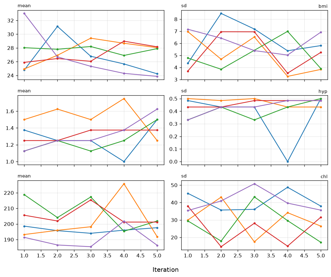

Python (PyMICE)

4. Change imputation method — v02_trace_nhanes2.png

R (Reference)

5. Extended iteration trace

Step parity: ✅ MATCH (0 exact, 0 info, 1 visual, 0 skipped, 0 mismatch of 1 blocks)

Though using just five iterations (the default) often works well in practice, we need to extend the number of iterations of the mice algorithm to confirm that there is no trend and that the trace lines intermingle well. We can increase the number of iterations to 40 by running 35 additional iterations using the mice.mids() function.

Note: 40-iteration trace via continue_imputation(imp3, maxit=35).

Python (PyMICE)

plot_mids(imp40, variables=['bmi', 'hyp', 'chl'])

Console Output

(plot below)

R (Reference)

imp40 <- mice.mids(imp, maxit=35, print=F)
plot(imp40)

plot_mids(imp40, variables=['bmi', 'hyp', 'chl'])

Console Output

(plot below)

imp40 <- mice.mids(imp, maxit=35, print=F)
plot(imp40)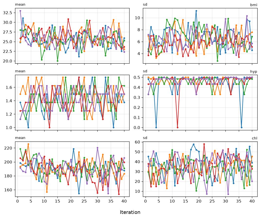

Python (PyMICE)

5. Extended iteration trace — v02_trace_40.png

R (Reference)

6. Stripplot diagnostics

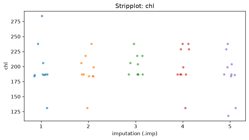
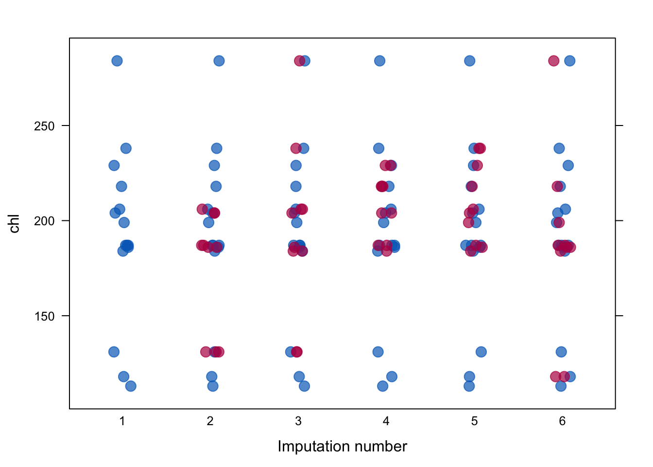
Step parity: ✅ MATCH (0 exact, 0 info, 2 visual, 0 skipped, 0 mismatch of 2 blocks)

Generally, one would prefer for the imputed data to be plausible values, i.e. values that could have been observed if they had not been missing. In order to form an idea about plausibility, one may check the imputations and compare them against the observed values. If we are willing to assume that the data are missing completely at random (MCAR), then the imputations should have the same distribution as the observed data. In general, distributions may be different because the missing data are MAR (or even MNAR). However, very large discrepancies need to be screened. Let us plot the observed and imputed data of chl by

Note: Matplotlib equivalent of the R lattice plot.

Python (PyMICE)

fig = plot_stripplot(imp3, 'chl')
save_figure(fig, ASSETS, 'v02_stripplot.png')

Console Output

(plot below)

R (Reference)

stripplot(imp, chl~.imp, pch=20, cex=2)

fig = plot_stripplot(imp3, 'chl')
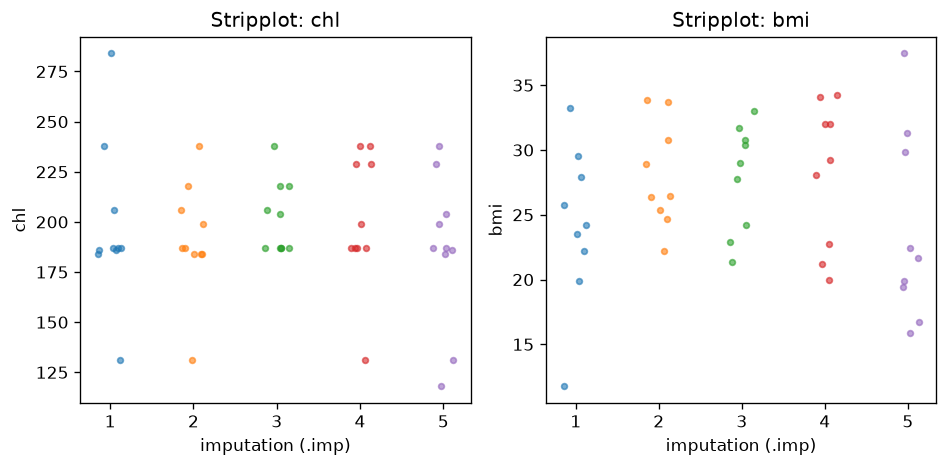
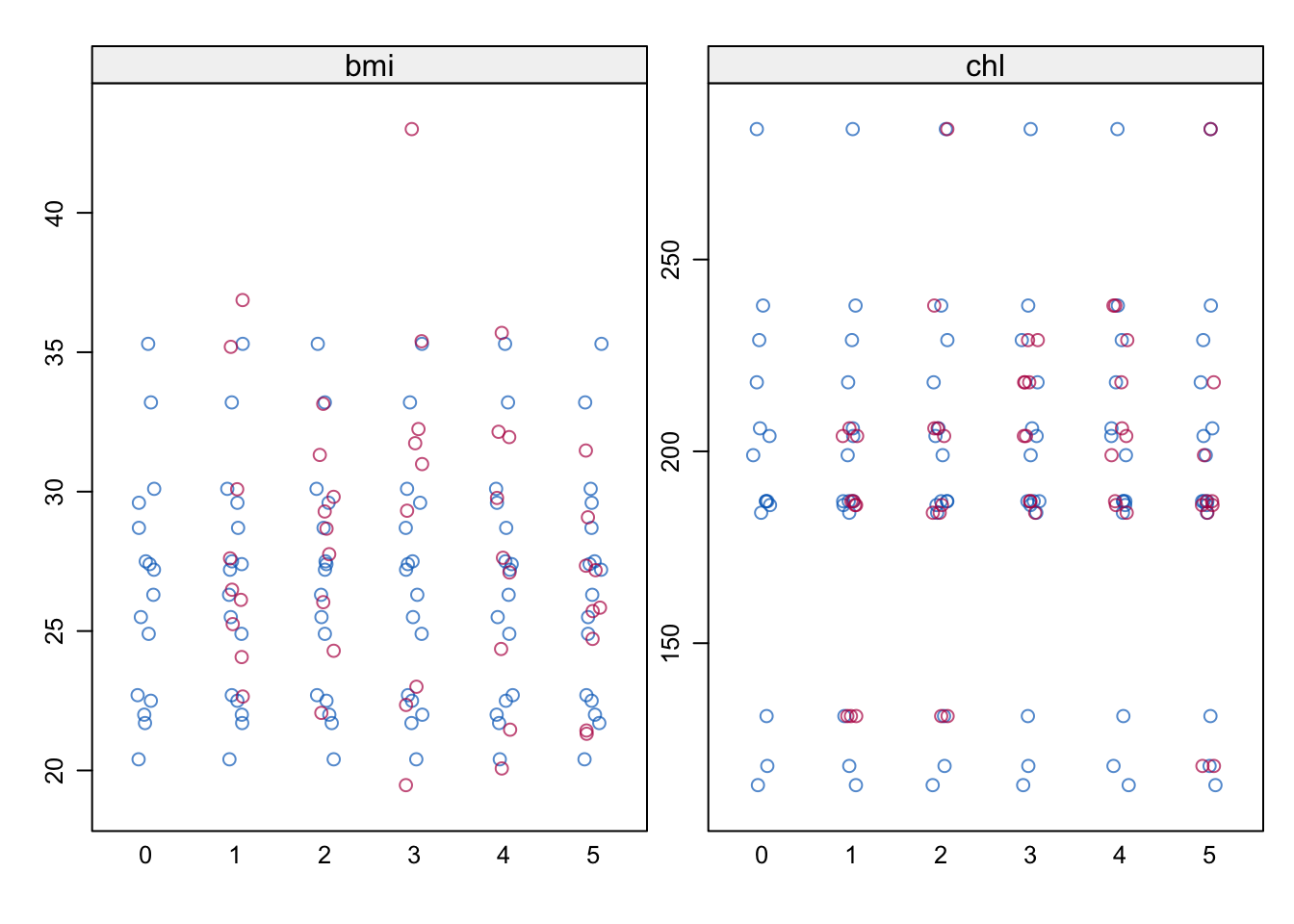
save_figure(fig, ASSETS, 'v02_stripplot.png')

Console Output

(plot below)

stripplot(imp, chl~.imp, pch=20, cex=2)

The convention is to plot observed data in blue and the imputed data in red. The figure graphs the data values of chl before and after imputation. Since the PMM method draws imputations from the observed data, imputed values have the same gaps as in the observed data, and are always within the range of the observed data. The figure indicates that the distributions of the imputed and the observed values are similar. The observed data have a particular feature that, for some reason, the data cluster around the value of 187. The imputations reflect this feature, and are close to the data. Under MCAR, univariate distributions of the observed and imputed data are expected to be identical. Under MAR, they can be different, both in location and spread, but their multivariate distribution is assumed to be identical. There are many other ways to look at the imputed data.

The following command creates a simpler version of the graph from the previous step and adds the plot for bmi.

Note: Matplotlib equivalent of the R lattice plot.

Python (PyMICE)

_stripplot_panel(imp3, ['chl', 'bmi'])

Console Output

(plot below)

R (Reference)

stripplot(imp)

_stripplot_panel(imp3, ['chl', 'bmi'])

Console Output

(plot below)

stripplot(imp)

Remember that bmi was imputed by Bayesian linear regression and (the range of) imputed values may therefore be different than observed values.

Python (PyMICE)

6. Stripplot diagnostics — v02_stripplot_chl.png

R (Reference)

Python (PyMICE)

R (Reference)

Repeated analysis in mice

7. Pooled regression fit

Step parity: ✅ MATCH (4 exact, 0 info, 0 visual, 0 skipped, 0 mismatch of 4 blocks)

Regression model on each completed dataset:

bmi = β₀ + β₁ chl + ε

Python (PyMICE)

print(format_mira_print_r(fit, nmis=imp3.nmis))

Console output (click to expand)

call :
with.mids(data = imp, expr = lm(bmi ~ chl))

call1 :
mice(data = nhanes2, method = meth, printFlag = F)

nmis :
age bmi hyp chl 
  0   9   8  10 

analyses :
[[1]]

Call:
lm(formula = bmi ~ chl)

Coefficients:
(Intercept)          chl  
     26.5370       -0.0042  

[[2]]

Call:
lm(formula = bmi ~ chl)

Coefficients:
(Intercept)          chl  
     21.2479        0.0305  

[[3]]

Call:
lm(formula = bmi ~ chl)

Coefficients:
(Intercept)          chl  
     20.6255        0.0328  

[[4]]

Call:
lm(formula = bmi ~ chl)

Coefficients:
(Intercept)          chl  
     22.2736        0.0249  

[[5]]

Call:
lm(formula = bmi ~ chl)

Coefficients:
(Intercept)          chl  
     18.3207        0.0384

R (Reference)

fit <- with(imp, lm(bmi ~ chl))
fit

R Console Output

call :
with.mids(data = imp, expr = lm(bmi ~ chl))

call1 :
mice(data = nhanes2, method = meth, printFlag = F)

nmis :
age bmi hyp chl 
  0   9   8  10 

analyses :
[[1]]

Call:
lm(formula = bmi ~ chl)

Coefficients:
(Intercept)          chl  
     26.5370       -0.0042  

[[2]]

Call:
lm(formula = bmi ~ chl)

Coefficients:
(Intercept)          chl  
     21.2479        0.0305  

[[3]]

Call:
lm(formula = bmi ~ chl)

Coefficients:
(Intercept)          chl  
     20.6255        0.0328  

[[4]]

Call:
lm(formula = bmi ~ chl)

Coefficients:
(Intercept)          chl  
     22.2736        0.0249  

[[5]]

Call:
lm(formula = bmi ~ chl)

Coefficients:
(Intercept)          chl  
     18.3207        0.0384

print(format_mira_print_r(fit, nmis=imp3.nmis))

Console output (click to expand)

call :
with.mids(data = imp, expr = lm(bmi ~ chl))

call1 :
mice(data = nhanes2, method = meth, printFlag = F)

nmis :
age bmi hyp chl 
  0   9   8  10 

analyses :
[[1]]

Call:
lm(formula = bmi ~ chl)

Coefficients:
(Intercept)          chl  
     26.5370       -0.0042  

[[2]]

Call:
lm(formula = bmi ~ chl)

Coefficients:
(Intercept)          chl  
     21.2479        0.0305  

[[3]]

Call:
lm(formula = bmi ~ chl)

Coefficients:
(Intercept)          chl  
     20.6255        0.0328  

[[4]]

Call:
lm(formula = bmi ~ chl)

Coefficients:
(Intercept)          chl  
     22.2736        0.0249  

[[5]]

Call:
lm(formula = bmi ~ chl)

Coefficients:
(Intercept)          chl  
     18.3207        0.0384

fit <- with(imp, lm(bmi ~ chl))
fit

R Console Output

call :
with.mids(data = imp, expr = lm(bmi ~ chl))

call1 :
mice(data = nhanes2, method = meth, printFlag = F)

nmis :
age bmi hyp chl 
  0   9   8  10 

analyses :
[[1]]

Call:
lm(formula = bmi ~ chl)

Coefficients:
(Intercept)          chl  
     26.5370       -0.0042  

[[2]]

Call:
lm(formula = bmi ~ chl)

Coefficients:
(Intercept)          chl  
     21.2479        0.0305  

[[3]]

Call:
lm(formula = bmi ~ chl)

Coefficients:
(Intercept)          chl  
     20.6255        0.0328  

[[4]]

Call:
lm(formula = bmi ~ chl)

Coefficients:
(Intercept)          chl  
     22.2736        0.0249  

[[5]]

Call:
lm(formula = bmi ~ chl)

Coefficients:
(Intercept)          chl  
     18.3207        0.0384

The fit object contains the regression summaries for each data set. The new object fit is actually of class mira (multiply imputed repeated analyses).

Python (PyMICE)

print('[1] "mira"   "matrix"')

Console Output

[1] "mira"   "matrix"

R (Reference)

class(fit)

R Console Output

[1] "mira"   "matrix"

print('[1] "mira"   "matrix"')

Console Output

[1] "mira"   "matrix"

class(fit)

R Console Output

[1] "mira"   "matrix"

Use the ls() function to what out what is in the object.

Python (PyMICE)

print('[1] "analyses" "call"     "call1"    "nmis"')

Console Output

[1] "analyses" "call"     "call1"    "nmis"

R (Reference)

ls(fit)

R Console Output

[1] "analyses" "call"     "call1"    "nmis"

print('[1] "analyses" "call"     "call1"    "nmis"')

Console Output

[1] "analyses" "call"     "call1"    "nmis"

ls(fit)

R Console Output

[1] "analyses" "call"     "call1"    "nmis"

Suppose we want to find the regression model fitted to the second imputed data set. It can be found as

Python (PyMICE)

filled2 = complete(imp3, 2)
print(format_lm_summary_r('bmi ~ chl', filled2, names2))

Console Output

Call:
lm(formula = bmi ~ chl)

Residuals:
    Min      1Q  Median      3Q     Max 
  -6.5111   -2.5430   -0.3816    2.6453    7.3992 

Coefficients:
            Estimate Std. Error t value Pr(>|t|)  
(Intercept)  21.24786    4.19493   5.065  0.0000 ***
chl           0.03052    0.02149   1.420  0.1689  
---
Signif. codes:  0 '***' 0.001 '**' 0.01 '*' 0.05 '.' 0.1 ' ' 1

Residual standard error: 4.0552 on 23 degrees of freedom
Multiple R-squared:  0.0806, Adjusted R-squared:  0.04067 
F-statistic: 2.018 on 1 and 23 DF,  p-value: 0.1689

R (Reference)

summary(fit$analyses[[2]])

R Console Output

Call:
lm(formula = bmi ~ chl)

Residuals:
    Min      1Q  Median      3Q     Max 
  -6.5111   -2.5430   -0.3816    2.6453    7.3992 

Coefficients:
            Estimate Std. Error t value Pr(>|t|)  
(Intercept)  21.24786    4.19493   5.065  0.0000 ***
chl           0.03052    0.02149   1.420  0.1689  
---
Signif. codes:  0 '***' 0.001 '**' 0.01 '*' 0.05 '.' 0.1 ' ' 1

Residual standard error: 4.0552 on 23 degrees of freedom
Multiple R-squared:  0.0806, Adjusted R-squared:  0.04067 
F-statistic: 2.018 on 1 and 23 DF,  p-value: 0.1689

filled2 = complete(imp3, 2)
print(format_lm_summary_r('bmi ~ chl', filled2, names2))

Console Output

Call:
lm(formula = bmi ~ chl)

Residuals:
    Min      1Q  Median      3Q     Max 
  -6.5111   -2.5430   -0.3816    2.6453    7.3992 

Coefficients:
            Estimate Std. Error t value Pr(>|t|)  
(Intercept)  21.24786    4.19493   5.065  0.0000 ***
chl           0.03052    0.02149   1.420  0.1689  
---
Signif. codes:  0 '***' 0.001 '**' 0.01 '*' 0.05 '.' 0.1 ' ' 1

Residual standard error: 4.0552 on 23 degrees of freedom
Multiple R-squared:  0.0806, Adjusted R-squared:  0.04067 
F-statistic: 2.018 on 1 and 23 DF,  p-value: 0.1689

summary(fit$analyses[[2]])

R Console Output

Call:
lm(formula = bmi ~ chl)

Residuals:
    Min      1Q  Median      3Q     Max 
  -6.5111   -2.5430   -0.3816    2.6453    7.3992 

Coefficients:
            Estimate Std. Error t value Pr(>|t|)  
(Intercept)  21.24786    4.19493   5.065  0.0000 ***
chl           0.03052    0.02149   1.420  0.1689  
---
Signif. codes:  0 '***' 0.001 '**' 0.01 '*' 0.05 '.' 0.1 ' ' 1

Residual standard error: 4.0552 on 23 degrees of freedom
Multiple R-squared:  0.0806, Adjusted R-squared:  0.04067 
F-statistic: 2.018 on 1 and 23 DF,  p-value: 0.1689

8. Pool multiply imputed model

Step parity: ✅ MATCH (1 exact, 0 info, 0 visual, 0 skipped, 0 mismatch of 1 blocks)

Pooling the repeated regression analyses can be done simply by typing

Python (PyMICE)

pooled = pool(fit)
print(format_pool_v02_r(summary_pool(pooled)))

Console Output

              estimate  std.error statistic       df     p.value
(Intercept)  21.8009113 5.74829615  3.792587 10.22632 0.003390551
chl          0.0244790 0.03010637  0.813085 9.14210 0.436831810

R (Reference)

pool.fit <- pool(fit)
summary(pool.fit)

R Console Output

              estimate  std.error statistic       df     p.value
(Intercept)  21.8009113 5.74829615  3.792587 10.22632 0.003390551
chl          0.0244790 0.03010637  0.813085 9.14210 0.436831810

pooled = pool(fit)
print(format_pool_v02_r(summary_pool(pooled)))

Console Output

              estimate  std.error statistic       df     p.value
(Intercept)  21.8009113 5.74829615  3.792587 10.22632 0.003390551
chl          0.0244790 0.03010637  0.813085 9.14210 0.436831810

pool.fit <- pool(fit)
summary(pool.fit)

R Console Output

              estimate  std.error statistic       df     p.value
(Intercept)  21.8009113 5.74829615  3.792587 10.22632 0.003390551
chl          0.0244790 0.03010637  0.813085 9.14210 0.436831810

which gives the relevant pooled regression coefficients and parameters, as well as the fraction of information about the coefficients missing due to nonresponse (fmi) and the proportion of the variation attributable to the missing data (lambda). The pooled fit object is of class mipo, which stands for multiply imputed pooled object.

mice is able to pool many analyses from a variety of packages for you, as long as the functions adhere to the coef method convention in R. For flexibility and in order to run custom pooling functions, mice also incorporates a function pool.scalar() which pools univariate estimates of m repeated complete data analysis conform Rubin's pooling rules (Rubin, 1987, paragraph 3.1)