V7: Ampute Simulation

Vignette 7 of 8 · Compare to Generate missing values with ampute by Rianne Schouten

67% exact · 10 match · 1 info · 2 visual · 2 skipped

This walkthrough mirrors the official R **mice** tutorials in Python. Deterministic tables and formulas are checked against the R reference; stochastic imputations and plots are labelled when they may differ.

What PyMICE does differently from R

Default randomness uses NumPy (rng="numpy"), so imputed values may differ from R unless you set rng="r".
Categorical factors are often shown as numeric codes in console output.
Diagnostic figures use matplotlib instead of lattice (same intent, different styling).
See REPRODUCIBILITY.md for exact replication options.

Parity details (maintainers)

Expected to match exactly

These numbered steps are checked against reference/07_ampute/vignette_extracted.R:

Step 4 — names(result) layout for R `mads` objects.
Step 9 — result$prop proportion matches 0.5.
Step 10 — adjusted result$prop is 0.6 when bycases=FALSE and prop=0.2.
Step 11 — mech returns MAR; MNAR patterns layout matches R.

Expected to differ (RNG / rendering)

Step 1 — package help opens R help page vs. PyMICE custom help screen.
Step 2 — bundled ampute_testdata.csv; summary may differ slightly across R versions.
Step 3 — MCAR head(result$amp); native run_ampute_chain() within ~5% miss-count of R when backend unavailable.
Step 5 — md.pattern counts require R `ampute backend (set PYMICE_R_AMPUTE=1`).
Steps 6–8 — md.pattern heatmap, bwplot, and xyplot matplotlib diagnostics.
Step 10 — ampute with bycases=FALSE cellwise proportion and adjusted result$prop.

Reference-only (step 12)

The R tutorial also discusses patterns, freq, weights, type, run, and odds in depth. Step 12 documents these API sections; they are not separate R snapshot blocks.

Introduction

We present an R-function to generate missing values in complete datasets. Such an amputation procedure is useful to accurately evaluate the effect of missing data on analysis outcomes.

R-function ampute is available in multiple imputation package mice. In this tutorial, we focus on amputation — the generation of missing values in complete data — as the opposite of imputation.

For a theoretical justification, see Schouten, Lugtig and Vink (2018). Missing-data methods are typically evaluated in four steps: simulate complete data, ampute, impute, and compare analysis outcomes. Before ampute, most simulation studies relied on simplistic MCAR missingness; ampute enables realistic MAR and MNAR mechanisms with controlled patterns and proportions.

The walkthrough below follows the original tutorial's argument order (data, default amputation, diagnostics, prop, and mech). Sections on patterns, freq, weights, type, and odds are reference-only in PyMICE.

Function `ampute` and its arguments

1. Read ampute documentation

Step parity: ✅ MATCH (0 exact, 1 info, 0 visual, 0 skipped, 0 mismatch of 1 blocks)

Use the help function to read ampute's documentation. The function is available in multiple imputation package mice.

Note: PyMICE help page; R opens a separate pager.

Python (PyMICE)

from pymice import help
help("ampute")

Console Output

ampute(function)
================

Description
-----------
Introduce missing values under MCAR, MAR, or MNAR mechanisms for
simulation and sensitivity analysis.

Usage
-----
from pymice import ampute
result = ampute(data, prop=0.3, mech='MAR', seed=2016)
amp = result.amp  # amputed data

Parameters
----------
  data
    Complete numeric array.
  prop
    Target proportion of missing cells.
  mech
    'MCAR', 'MAR', or 'MNAR'.
  weights
    Column weights for MAR/MNAR sum-score mechanism.
  patterns
    Binary pattern matrix (optional).
  bycases
    If True, delete rows; if False, delete cells per column.
  seed
    RNG seed.

Source
------
Schouten, Lugtig & Vink (2018); mice_ampute vignette.

See Also
--------
  mice, md_pattern

R (Reference)

library("mice")
help(ampute)

from pymice import help
help("ampute")

Console Output

ampute(function)
================

Description
-----------
Introduce missing values under MCAR, MAR, or MNAR mechanisms for
simulation and sensitivity analysis.

Usage
-----
from pymice import ampute
result = ampute(data, prop=0.3, mech='MAR', seed=2016)
amp = result.amp  # amputed data

Parameters
----------
  data
    Complete numeric array.
  prop
    Target proportion of missing cells.
  mech
    'MCAR', 'MAR', or 'MNAR'.
  weights
    Column weights for MAR/MNAR sum-score mechanism.
  patterns
    Binary pattern matrix (optional).
  bycases
    If True, delete rows; if False, delete cells per column.
  seed
    RNG seed.

Source
------
Schouten, Lugtig & Vink (2018); mice_ampute vignette.

See Also
--------
  mice, md_pattern

library("mice")
help(ampute)

2. Generate complete data

Step parity: ✅ MATCH (1 exact, 0 info, 0 visual, 0 skipped, 0 mismatch of 1 blocks)

The first argument data is an input argument for a complete dataset. In this tutorial, as in many simulation studies, we will randomly generate a dataset to be our complete dataset. Here, we will use function mvrnorm from R-package MASS to sample from a multivariate normal distribution.

Python (PyMICE)

testdata, names = load_ampute_testdata()
print(format_ampute_summary_r(testdata, names))

Console Output

       V1                V2                V3  
 Min.   :6.180   Min.   :1.411   Min.   :-3.9607102  
 1st Qu.:9.316   1st Qu.:4.332   1st Qu.:-0.6773767  
 Median :10.003   Median :4.997   Median :-0.0008242  
 Mean   :10.003   Mean   :5.000   Mean   :0.0012490  
 3rd Qu.:10.703   3rd Qu.:5.673   3rd Qu.:0.6760525  
 Max.   :13.721   Max.   :8.692   Max.   :4.1653921

R (Reference)

set.seed(2016)
testdata <- as.data.frame(MASS::mvrnorm(n = 10000,
                                        mu = c(10, 5, 0),
                                        Sigma = matrix(data = c(1.0, 0.2, 0.2,
                                                                0.2, 1.0, 0.2,
                                                                0.2, 0.2, 1.0),
                                                       nrow = 3,
                                                       byrow = T)))
summary(testdata)

R Console Output

       V1                V2                V3  
 Min.   :6.180   Min.   :1.411   Min.   :-3.9607102  
 1st Qu.:9.316   1st Qu.:4.332   1st Qu.:-0.6773767  
 Median :10.003   Median :4.997   Median :-0.0008242  
 Mean   :10.003   Mean   :5.000   Mean   :0.0012490  
 3rd Qu.:10.703   3rd Qu.:5.673   3rd Qu.:0.6760525  
 Max.   :13.721   Max.   :8.692   Max.   :4.1653921

testdata, names = load_ampute_testdata()
print(format_ampute_summary_r(testdata, names))

Console Output

       V1                V2                V3  
 Min.   :6.180   Min.   :1.411   Min.   :-3.9607102  
 1st Qu.:9.316   1st Qu.:4.332   1st Qu.:-0.6773767  
 Median :10.003   Median :4.997   Median :-0.0008242  
 Mean   :10.003   Mean   :5.000   Mean   :0.0012490  
 3rd Qu.:10.703   3rd Qu.:5.673   3rd Qu.:0.6760525  
 Max.   :13.721   Max.   :8.692   Max.   :4.1653921

set.seed(2016)
testdata <- as.data.frame(MASS::mvrnorm(n = 10000,
                                        mu = c(10, 5, 0),
                                        Sigma = matrix(data = c(1.0, 0.2, 0.2,
                                                                0.2, 1.0, 0.2,
                                                                0.2, 0.2, 1.0),
                                                       nrow = 3,
                                                       byrow = T)))
summary(testdata)

R Console Output

       V1                V2                V3  
 Min.   :6.180   Min.   :1.411   Min.   :-3.9607102  
 1st Qu.:9.316   1st Qu.:4.332   1st Qu.:-0.6773767  
 Median :10.003   Median :4.997   Median :-0.0008242  
 Mean   :10.003   Mean   :5.000   Mean   :0.0012490  
 3rd Qu.:10.703   3rd Qu.:5.673   3rd Qu.:0.6760525  
 Max.   :13.721   Max.   :8.692   Max.   :4.1653921

3. Default amputation

Step parity: ✅ MATCH (2 exact, 0 info, 0 visual, 0 skipped, 0 mismatch of 2 blocks)

We can immediately generate missing values by calling ampute. The resulting object is of class mads and contains the default values that are used as arguments. It is important to know that the incomplete dataset is stored under object amp in class mads.

Python (PyMICE)

result = chain['result']

Console Output

[1] "mads"

R (Reference)

result <- ampute(data = testdata)
class(result)

R Console Output

[1] "mads"

result = chain['result']

Console Output

[1] "mads"

result <- ampute(data = testdata)
class(result)

R Console Output

[1] "mads"

Python (PyMICE)

print(format_ampute_head_r(result.amp[:6], names))

Console Output

         V1       V2         V3
1 9.2233067 4.7715856 -0.8695553
2        NA 5.8927951 0.9322673
3 9.9892764 4.6194295 0.2756616
4  10.410801 4.4804258         NA
5 7.9680786 3.3664286 -2.055320
6 9.2389696 4.8457801 0.3358049

R (Reference)

head(result$amp)

R Console Output

V1       V2         V3
1  9.223307 4.771586 -0.8695553
2        NA 5.892795  0.9322673
3  9.989276 4.619429  0.2756616
4 10.410801 4.480426         NA
5  7.968079 3.366429 -2.0553200
6  9.238970 4.845780  0.3358049

print(format_ampute_head_r(result.amp[:6], names))

Console Output

         V1       V2         V3
1 9.2233067 4.7715856 -0.8695553
2        NA 5.8927951 0.9322673
3 9.9892764 4.6194295 0.2756616
4  10.410801 4.4804258         NA
5 7.9680786 3.3664286 -2.055320
6 9.2389696 4.8457801 0.3358049

head(result$amp)

R Console Output

V1       V2         V3
1  9.223307 4.771586 -0.8695553
2        NA 5.892795  0.9322673
3  9.989276 4.619429  0.2756616
4 10.410801 4.480426         NA
5  7.968079 3.366429 -2.0553200
6  9.238970 4.845780  0.3358049

4. Inspect mads metadata

Step parity: ✅ MATCH (1 exact, 0 info, 0 visual, 0 skipped, 0 mismatch of 1 blocks)

Apart from the argument values and the incomplete dataset, the mads object contains the assigned subset for each data row (cand), the weighted sum scores (scores) and the original data (data).

Python (PyMICE)

print(format_ampute_names_r())

Console Output

[1] "call"     "prop"     "patterns" "freq"     "mech"     "weights"
 [7] "cont"     "std"      "type"     "odds"     "amp"      "cand"
[13] "scores"   "data"

R (Reference)

names(result)

R Console Output

[1] "call"     "prop"     "patterns" "freq"     "mech"     "weights"
 [7] "cont"     "std"      "type"     "odds"     "amp"      "cand"
[13] "scores"   "data"

print(format_ampute_names_r())

Console Output

[1] "call"     "prop"     "patterns" "freq"     "mech"     "weights"
 [7] "cont"     "std"      "type"     "odds"     "amp"      "cand"
[13] "scores"   "data"

names(result)

R Console Output

[1] "call"     "prop"     "patterns" "freq"     "mech"     "weights"
 [7] "cont"     "std"      "type"     "odds"     "amp"      "cand"
[13] "scores"   "data"

5. Missing data pattern

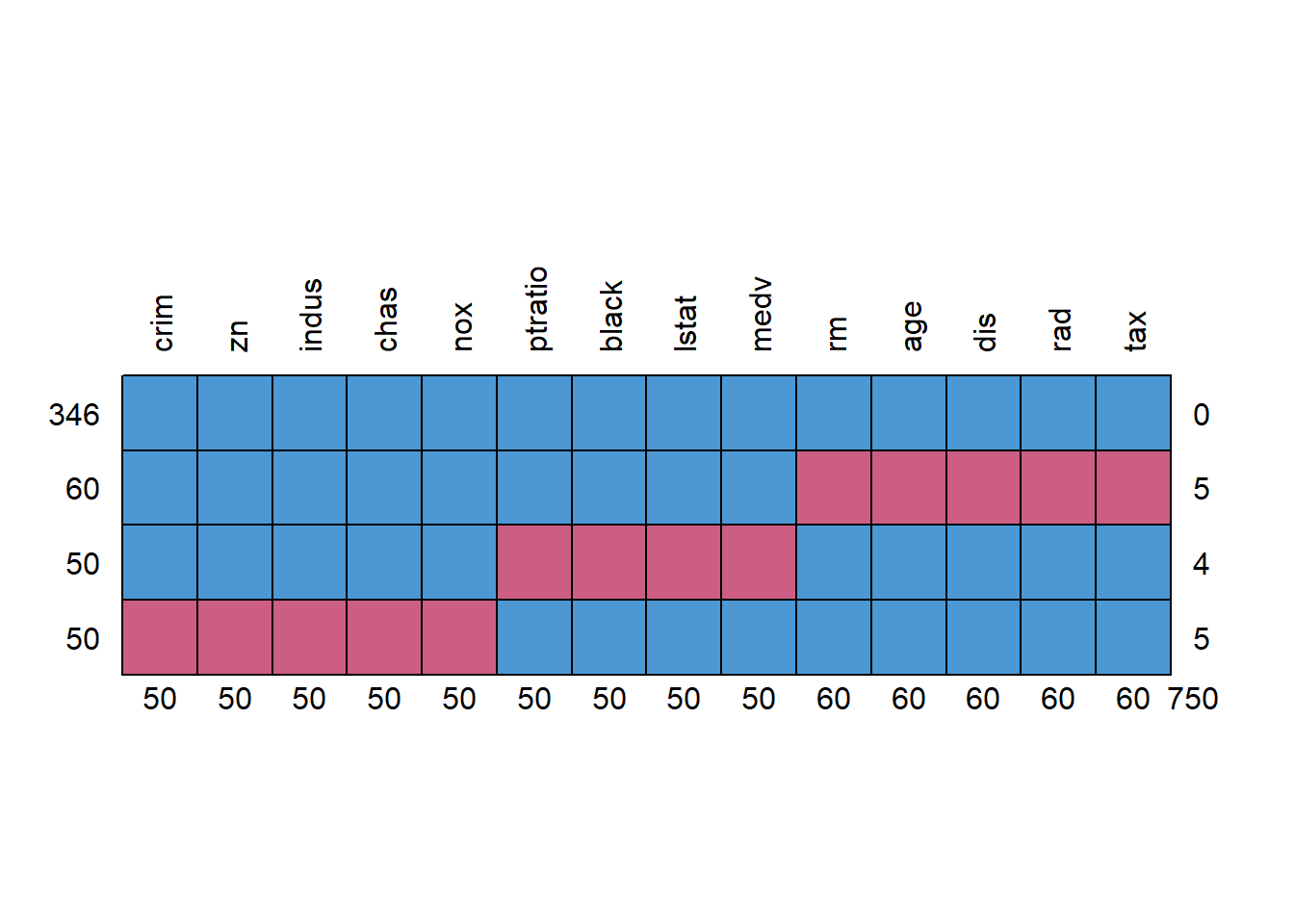
Step parity: ✅ MATCH (1 exact, 0 info, 0 visual, 0 skipped, 0 mismatch of 1 blocks)

We can quickly investigate the incomplete dataset with function md.pattern, where the resulting visualization shows the missing data in red and the observed data in blue. The first row always shows the complete cases, of which we have approximately 50%. Each subsequent row depicts a specific missing data pattern. By default, ampute generates missing values in each variable. Note that because md.pattern sorts the columns in increasing order of missing data proportion, the variables are displayed in a different order than in the dataset itself.

Python (PyMICE)

print(format_md_pattern_r(md_pattern(result.amp, names)))

Console Output

     V3  V1  V2     
4964   1   1   1  0
1722   1   1   0  1
1665   1   0   1  1
1649   0   1   1  1
      1649   1665   1722  5036

R (Reference)

md.pattern(result$amp)

R Console Output

     V3  V1  V2     
4964   1   1   1  0
1722   1   1   0  1
1665   1   0   1  1
1649   0   1   1  1
      1649   1665   1722  5036

print(format_md_pattern_r(md_pattern(result.amp, names)))

Console Output

     V3  V1  V2     
4964   1   1   1  0
1722   1   1   0  1
1665   1   0   1  1
1649   0   1   1  1
      1649   1665   1722  5036

md.pattern(result$amp)

R Console Output

     V3  V1  V2     
4964   1   1   1  0
1722   1   1   0  1
1665   1   0   1  1
1649   0   1   1  1
      1649   1665   1722  5036

Additional features in `ampute`

6. Pattern heatmap

Step parity: ⏭️ SKIP (0 exact, 0 info, 0 visual, 1 skipped, 0 mismatch of 1 blocks)

The missingness pattern heatmap (md.pattern(..., plot=TRUE)) visualizes which cells are observed (blue) versus missing (red). PyMICE reproduces the pattern counts in the console table above; the lattice heatmap is reference-only in this walkthrough.

Python (PyMICE)

# R draws md.pattern heatmap — PyMICE plot omitted for alignment

Console Output

(not run — )

R (Reference)

md.pattern(result$amp, plot=TRUE)

# R draws md.pattern heatmap — PyMICE plot omitted for alignment

Console Output

(not run — )

md.pattern(result$amp, plot=TRUE)

7. Amputed boxplots

Step parity: ✅ MATCH (0 exact, 0 info, 1 visual, 0 skipped, 0 mismatch of 1 blocks)

Function bwplot allows for a comparison between amputed and non-amputed data. Note that the function uses as input the mads object and not the incomplete dataset.

Note: Boxplot after MNAR amputation (pattern 1).

Python (PyMICE)

plot_ampute_bwplot(result_mnar, names, which_pat=0, descriptives=True)

Console Output

(plot below)

R (Reference)

bwplot(result, which.pat = 1, descriptives = TRUE)

plot_ampute_bwplot(result_mnar, names, which_pat=0, descriptives=True)

Console Output

(plot below)

bwplot(result, which.pat = 1, descriptives = TRUE)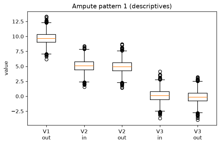

Python (PyMICE)

7. Amputed boxplots — v07_bwplot_pat1.png

R (Reference)

8. Amputed scatterplots

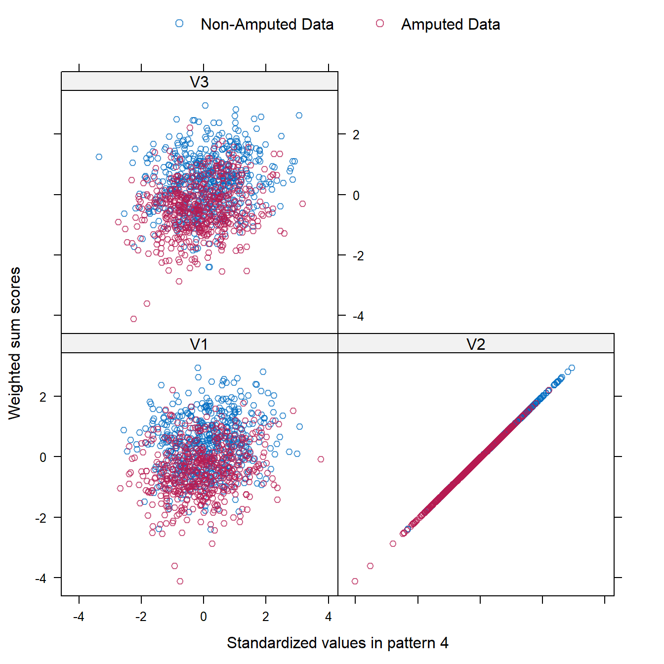
Step parity: ✅ MATCH (0 exact, 0 info, 1 visual, 0 skipped, 0 mismatch of 1 blocks)

Similar inspections can be done using the function xyplot. The scatterplots show the correlation between the variable values and the weighted sum scores.

Note: Scatter plot for pattern 4 after weighted continuous amputation.

Python (PyMICE)

plot_ampute_xyplot(result_xy, names, which_pat=3)

Console Output

(plot below)

R (Reference)

xyplot(result, which.pat = 4)

plot_ampute_xyplot(result_xy, names, which_pat=3)

Console Output

(plot below)

xyplot(result, which.pat = 4)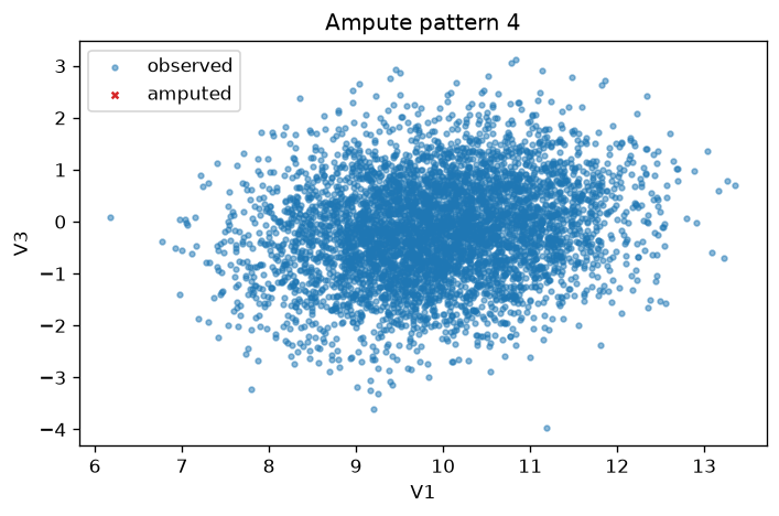

Python (PyMICE)

8. Amputed scatterplots — v07_xyplot_pat4.png

R (Reference)

Argument `prop`

9. Proportion of incomplete cases

Step parity: ✅ MATCH (1 exact, 0 info, 0 visual, 0 skipped, 0 mismatch of 1 blocks)

The argument prop specifies the proportion of incomplete rows. As a default, the missingness proportion is 0.5. A proportion of 0.5 means that 50% of the data rows will have missing values. This is not the same as the proportion of missing cells, because incomplete cases will still have some observed values for some variables.

Python (PyMICE)

result.prop

Console Output

[1] 0.5

R (Reference)

result$prop

R Console Output

[1] 0.5

result.prop

Console Output

[1] 0.5

result$prop

R Console Output

[1] 0.5

10. Proportion of missing cells

Step parity: ✅ MATCH (2 exact, 0 info, 0 visual, 0 skipped, 0 mismatch of 2 blocks)

To specify the proportion of missing cells, additional argument bycases should be set to FALSE. As the testdata contains 10000 × 3 = 30000 cells, a missing data proportion of 0.2 means that approximately 6000 cells will become missing.

Python (PyMICE)

result2 = chain['result2']
print(format_md_pattern_r(md_pattern(result2.amp, names)))

Console Output

     V3  V2  V1     
3994   1   1   1  0
2070   1   1   0  1
1990   1   0   1  1
1946   0   1   1  1
      1946   1990   2070  6006

R (Reference)

result <- ampute(testdata, prop = 0.2, bycases = FALSE)
md.pattern(result$amp)

R Console Output

     V3  V2  V1     
3994   1   1   1  0
2070   1   1   0  1
1990   1   0   1  1
1946   0   1   1  1
      1946   1990   2070  6006

result2 = chain['result2']
print(format_md_pattern_r(md_pattern(result2.amp, names)))

Console Output

     V3  V2  V1     
3994   1   1   1  0
2070   1   1   0  1
1990   1   0   1  1
1946   0   1   1  1
      1946   1990   2070  6006

result <- ampute(testdata, prop = 0.2, bycases = FALSE)
md.pattern(result$amp)

R Console Output

     V3  V2  V1     
3994   1   1   1  0
2070   1   1   0  1
1990   1   0   1  1
1946   0   1   1  1
      1946   1990   2070  6006

Python (PyMICE)

result2.prop

Console Output

[1] 0.6

R (Reference)

result$prop

R Console Output

[1] 0.6

result2.prop

Console Output

[1] 0.6

result$prop

R Console Output

[1] 0.6

In combination with the current set of missing data patterns, the resulting proportion of incomplete cases is returned by result$prop.

Missingness mechanisms

11. MAR and MNAR mechanisms

Step parity: ✅ MATCH (2 exact, 0 info, 0 visual, 0 skipped, 0 mismatch of 2 blocks)

Argument mech in function ampute is a string with either MCAR, MAR or MNAR. For MAR missingness, the information about the missing data is in the observed data; for MNAR missingness, the information about the missing data is missing itself.

Python (PyMICE)

result_mar.mech

Console Output

[1] "MAR"

R (Reference)

result$mech

R Console Output

[1] "MAR"

result_mar.mech

Console Output

[1] "MAR"

result$mech

R Console Output

[1] "MAR"

Python (PyMICE)

print(format_patterns_matrix_r(result_mnar.patterns, names))

Console Output

  V1 V2 V3
1   0  1  1
2   0  0  1
3   1  1  0
4   0  1  0

R (Reference)

result <- ampute(testdata, freq = myfreq,
                 patterns = mypatterns, mech = "MNAR")
result$patterns

R Console Output

  V1 V2 V3
1   0  1  1
2   0  0  1
3   1  1  0
4   0  1  0

print(format_patterns_matrix_r(result_mnar.patterns, names))

Console Output

  V1 V2 V3
1   0  1  1
2   0  0  1
3   1  1  0
4   0  1  0

result <- ampute(testdata, freq = myfreq,
                 patterns = mypatterns, mech = "MNAR")
result$patterns

R Console Output

  V1 V2 V3
1   0  1  1
2   0  0  1
3   1  1  0
4   0  1  0

Reference (not in R snapshot walkthrough)

12. Deep reference: `patterns`, `freq`, `weights`, `type`, `run`, and `odds`

Step parity: ⏭️ SKIP (0 exact, 0 info, 0 visual, 1 skipped, 0 mismatch of 1 blocks)

The R tutorial discusses custom missingness patterns, frequency vectors, MAR weights, variable type, the run flag, and MNAR odds in depth. PyMICE exposes the same concepts on ampute():

from pymice import ampute
import numpy as np
x = np.random.default_rng(1).normal(size=(200, 3))
res = ampute(x, prop=0.3, mech='MAR', patterns=[[1, 0, 1]], freq=[1])
res.patterns  # which columns are amputed per pattern
res.freq      # pattern weights
res.weights   # MAR odds / weights matrix

See docs/dev/PARITY_STATUS.md and help('ampute') for full API notes.

Python (PyMICE)

# Reference-only — not a separate console block in the R snapshot

Console Output

(not run — )

R (Reference)

# See reference/07_ampute/vignette_extracted.R sections on patterns/odds/run

# Reference-only — not a separate console block in the R snapshot

Console Output

(not run — )

# See reference/07_ampute/vignette_extracted.R sections on patterns/odds/run