V3: Missingness Models
Vignette 3 of 8 · Compare to The imputation and nonresponse models by Gerko Vink and Stef van Buuren
This walkthrough mirrors the official R **mice** tutorials in Python. Deterministic tables and formulas are checked against the R reference; stochastic imputations and plots are labelled when they may differ.
What PyMICE does differently from R
- Default randomness uses NumPy (
rng="numpy"), so imputed values may differ from R unless you setrng="r". - Categorical factors are often shown as numeric codes in console output.
- Diagnostic figures use matplotlib instead of lattice (same intent, different styling).
- See REPRODUCIBILITY.md for exact replication options.
Parity details (maintainers)
Expected to match exactly
These numbered steps are checked against reference/03_missingness_inspection/vignette_extracted.R:
- Step 3 —
head(boys)with R row names;nrow(boys)→ 748;summary(boys)horizontal factor layout - Step 4 —
md.pattern(boys)pattern matrix - Step 5 —
sum(mpat[,"gen"]==0)→ 8 - Step 6 —
R <- is.na(boys$gen)logical vector print - Step 9 —
help('mammalsleep')R pager snapshot;head(mammalsleep)species labels;str(mammalsleep)layout (static reference);summary(mammalsleep)species counts;md.pattern(mammalsleep)with species column - Steps 10 & 13 — logged-event warnings on session mammalsleep chain (29 / 19 events; numeric
speciescodes). - Steps 12 & 14 —
pool(fit)/summary(pool())on mammalsleep (sws ~ log10(bw) + odi).
Expected to differ (RNG / rendering)
- Step 1 — package load; no R console output to compare.
- Step 2 —
help('boys')R pager snapshot (static reference text).
- Step 6 —
histogram()matplotlib panels. - Step 8 —
summary(complete(imp1))on session PMM chain;with(imp1, mean(tv))TV means - Step 10 —
plot(imp)trace lines (matplotlib vs lattice). - Step 15 —
plot(impnew)convergence traces.
Introduction
This is the third vignette in a series of six.
In this vignette we will focus on analyzing the relation between the data and the missingness. For non-R users: In R one can simply call the helpfunction for a any specific function func by typing help(func). E.g. help(mice) directs you to the help page of the mice function.
1. Load packages and seed
Note: Package load step; no R console output to compare.
import numpy as np
from pymice import mice, complete, with_mids, pool, help, md_pattern, summary_pool
from pymice.diagnostics.plots import plot_histogram, plot_mids
from lib.data import load_boys_full_matrix, load_mammalsleep_full
from lib.viz import save_figure
from lib.r_style import (
    format_bool_vector_r,
    format_dataframe_r,
    format_md_pattern_r,
    format_pool_mipo_r,
    format_pool_v03_summary_r,
    format_summary_r,
    format_tv_means_tibble_r
)(setup — no console output)require(mice)
require(lattice)
set.seed(123)import numpy as np
from pymice import mice, complete, with_mids, pool, help, md_pattern, summary_pool
from pymice.diagnostics.plots import plot_histogram, plot_mids
from lib.data import load_boys_full_matrix, load_mammalsleep_full
from lib.viz import save_figure
from lib.r_style import (
format_bool_vector_r,
format_dataframe_r,
format_md_pattern_r,
format_pool_mipo_r,
format_pool_v03_summary_r,
format_summary_r,
format_tv_means_tibble_r
)(setup — no console output)require(mice)
require(lattice)
set.seed(123)We choose seed value 123. This is an arbitrary value; any value would be an equally good seed value. Fixing the random seed enables you (and others) to exactly replicate anything that involves random number generators. If you set the seed in your R instance to 123, you will get the exact same results and plots as we present in this document.
2. Inspect boys dataset
To learn more about the contents of the data, use one of the two following help commands:
Note: Truncated R help excerpt (full pager is very long).
print(format_help_r('boys', max_lines=32))boys package:mice R Documentation
_G_r_o_w_t_h _o_f _D_u_t_c_h _b_o_y_s
_D_e_s_c_r_i_p_t_i_o_n:
Height, weight, head circumference and puberty of 748 Dutch boys.
_F_o_r_m_a_t:
A data frame with 748 rows on the following 9 variables:
age Decimal age (0-21 years)
hgt Height (cm)
wgt Weight (kg)
bmi Body mass index
hc Head circumference (cm)
gen Genital Tanner stage (G1-G5)
phb Pubic hair (Tanner P1-P6)
tv Testicular volume (ml)
reg Region (north, east, west, south, city)
_D_e_t_a_i_l_s:
... (72 more lines — full R help page omitted)help(boys)
?boysboys package:mice R Documentation
_G_r_o_w_t_h _o_f _D_u_t_c_h _b_o_y_s
_D_e_s_c_r_i_p_t_i_o_n:
Height, weight, head circumference and puberty of 748 Dutch boys.
_F_o_r_m_a_t:
A data frame with 748 rows on the following 9 variables:
age Decimal age (0-21 years)
hgt Height (cm)
wgt Weight (kg)
bmi Body mass index
hc Head circumference (cm)
gen Genital Tanner stage (G1-G5)
phb Pubic hair (Tanner P1-P6)
tv Testicular volume (ml)
reg Region (north, east, west, south, city)
_D_e_t_a_i_l_s:
Random sample of 10\ Dutch growth references 1997. Variables ‘gen’
and ‘phb’ are ordered factors. ‘reg’ is a factor.
_S_o_u_r_c_e:
Fredriks, A.M,, van Buuren, S., Burgmeijer, R.J., Meulmeester JF,
Beuker, R.J., Brugman, E., Roede, M.J., Verloove-Vanhorick, S.P.,
Wit, J.M. (2000) Continuing positive secular growth change in The
Netherlands 1955-1997. _Pediatric Research_, *47*, 316-323.
Fredriks, A.M., van Buuren, S., Wit, J.M., Verloove-Vanhorick,
S.P. (2000). Body index measurements in 1996-7 compared with 1980.
_Archives of Disease in Childhood_, *82*, 107-112.
_E_x_a_m_p_l_e_s:
# create two imputed data sets
imp <- mice(boys, m = 1, maxit = 2)
z <- complete(imp, 1)
# create imputations for age <8yrs
plot(z$age, z$gen,
col = mdc(1:2)[1 + is.na(boys$gen)],
xlab = "Age (years)", ylab = "Tanner Stage Genital"
)
# figure to show that the default imputation method does not impute BMI
# consistently
plot(z$bmi, z$wgt / (z$hgt / 100)^2,
col = mdc(1:2)[1 + is.na(boys$bmi)],
xlab = "Imputed BMI", ylab = "Calculated BMI"
)
# also, BMI distributions are somewhat different
oldpar <- par(mfrow = c(1, 2))
MASS::truehist(z$bmi[!is.na(boys$bmi)],
h = 1, xlim = c(10, 30), ymax = 0.25,
col = mdc(1), xlab = "BMI observed"
)
MASS::truehist(z$bmi[is.na(boys$bmi)],
h = 1, xlim = c(10, 30), ymax = 0.25,
col = mdc(2), xlab = "BMI imputed"
)
par(oldpar)
# repair the inconsistency problem by passive imputation
meth <- imp$meth
meth["bmi"] <- "~I(wgt/(hgt/100)^2)"
pred <- imp$predictorMatrix
pred["hgt", "bmi"] <- 0
pred["wgt", "bmi"] <- 0
imp2 <- mice(boys, m = 1, maxit = 2, meth = meth, pred = pred)
z2 <- complete(imp2, 1)
# show that new imputations are consistent
plot(z2$bmi, z2$wgt / (z2$hgt / 100)^2,
col = mdc(1:2)[1 + is.na(boys$bmi)],
ylab = "Calculated BMI"
)
# and compare distributions
oldpar <- par(mfrow = c(1, 2))
MASS::truehist(z2$bmi[!is.na(boys$bmi)],
h = 1, xlim = c(10, 30), ymax = 0.25, col = mdc(1),
xlab = "BMI observed"
)
MASS::truehist(z2$bmi[is.na(boys$bmi)],
h = 1, xlim = c(10, 30), ymax = 0.25, col = mdc(2),
xlab = "BMI imputed"
)
par(oldpar)print(format_help_r('boys', max_lines=32))boys package:mice R Documentation
_G_r_o_w_t_h _o_f _D_u_t_c_h _b_o_y_s
_D_e_s_c_r_i_p_t_i_o_n:
Height, weight, head circumference and puberty of 748 Dutch boys.
_F_o_r_m_a_t:
A data frame with 748 rows on the following 9 variables:
age Decimal age (0-21 years)
hgt Height (cm)
wgt Weight (kg)
bmi Body mass index
hc Head circumference (cm)
gen Genital Tanner stage (G1-G5)
phb Pubic hair (Tanner P1-P6)
tv Testicular volume (ml)
reg Region (north, east, west, south, city)
_D_e_t_a_i_l_s:
... (72 more lines — full R help page omitted)help(boys)
?boysboys package:mice R Documentation
_G_r_o_w_t_h _o_f _D_u_t_c_h _b_o_y_s
_D_e_s_c_r_i_p_t_i_o_n:
Height, weight, head circumference and puberty of 748 Dutch boys.
_F_o_r_m_a_t:
A data frame with 748 rows on the following 9 variables:
age Decimal age (0-21 years)
hgt Height (cm)
wgt Weight (kg)
bmi Body mass index
hc Head circumference (cm)
gen Genital Tanner stage (G1-G5)
phb Pubic hair (Tanner P1-P6)
tv Testicular volume (ml)
reg Region (north, east, west, south, city)
_D_e_t_a_i_l_s:
Random sample of 10\ Dutch growth references 1997. Variables ‘gen’
and ‘phb’ are ordered factors. ‘reg’ is a factor.
_S_o_u_r_c_e:
Fredriks, A.M,, van Buuren, S., Burgmeijer, R.J., Meulmeester JF,
Beuker, R.J., Brugman, E., Roede, M.J., Verloove-Vanhorick, S.P.,
Wit, J.M. (2000) Continuing positive secular growth change in The
Netherlands 1955-1997. _Pediatric Research_, *47*, 316-323.
Fredriks, A.M., van Buuren, S., Wit, J.M., Verloove-Vanhorick,
S.P. (2000). Body index measurements in 1996-7 compared with 1980.
_Archives of Disease in Childhood_, *82*, 107-112.
_E_x_a_m_p_l_e_s:
# create two imputed data sets
imp <- mice(boys, m = 1, maxit = 2)
z <- complete(imp, 1)
# create imputations for age <8yrs
plot(z$age, z$gen,
col = mdc(1:2)[1 + is.na(boys$gen)],
xlab = "Age (years)", ylab = "Tanner Stage Genital"
)
# figure to show that the default imputation method does not impute BMI
# consistently
plot(z$bmi, z$wgt / (z$hgt / 100)^2,
col = mdc(1:2)[1 + is.na(boys$bmi)],
xlab = "Imputed BMI", ylab = "Calculated BMI"
)
# also, BMI distributions are somewhat different
oldpar <- par(mfrow = c(1, 2))
MASS::truehist(z$bmi[!is.na(boys$bmi)],
h = 1, xlim = c(10, 30), ymax = 0.25,
col = mdc(1), xlab = "BMI observed"
)
MASS::truehist(z$bmi[is.na(boys$bmi)],
h = 1, xlim = c(10, 30), ymax = 0.25,
col = mdc(2), xlab = "BMI imputed"
)
par(oldpar)
# repair the inconsistency problem by passive imputation
meth <- imp$meth
meth["bmi"] <- "~I(wgt/(hgt/100)^2)"
pred <- imp$predictorMatrix
pred["hgt", "bmi"] <- 0
pred["wgt", "bmi"] <- 0
imp2 <- mice(boys, m = 1, maxit = 2, meth = meth, pred = pred)
z2 <- complete(imp2, 1)
# show that new imputations are consistent
plot(z2$bmi, z2$wgt / (z2$hgt / 100)^2,
col = mdc(1:2)[1 + is.na(boys$bmi)],
ylab = "Calculated BMI"
)
# and compare distributions
oldpar <- par(mfrow = c(1, 2))
MASS::truehist(z2$bmi[!is.na(boys$bmi)],
h = 1, xlim = c(10, 30), ymax = 0.25, col = mdc(1),
xlab = "BMI observed"
)
MASS::truehist(z2$bmi[is.na(boys$bmi)],
h = 1, xlim = c(10, 30), ymax = 0.25, col = mdc(2),
xlab = "BMI imputed"
)
par(oldpar)3. Dataset size and missingness
print(format_boys_head_r()) age hgt wgt bmi hc gen phb tv reg
3 0.035 50.1 3.650 14.54 33.7 <NA> <NA> NA south
4 0.038 53.5 3.370 11.77 35.0 <NA> <NA> NA south
18 0.057 50.0 3.140 12.56 35.2 <NA> <NA> NA south
23 0.060 54.5 4.270 14.37 36.7 <NA> <NA> NA south
28 0.062 57.5 5.030 15.21 37.3 <NA> <NA> NA south
36 0.068 55.5 4.655 15.11 37.0 <NA> <NA> NA southhead(boys) age hgt wgt bmi hc gen phb tv reg
3 0.035 50.1 3.650 14.54 33.7 <NA> <NA> NA south
4 0.038 53.5 3.370 11.77 35.0 <NA> <NA> NA south
18 0.057 50.0 3.140 12.56 35.2 <NA> <NA> NA south
23 0.060 54.5 4.270 14.37 36.7 <NA> <NA> NA south
28 0.062 57.5 5.030 15.21 37.3 <NA> <NA> NA south
36 0.068 55.5 4.655 15.11 37.0 <NA> <NA> NA southprint(format_boys_head_r()) age hgt wgt bmi hc gen phb tv reg
3 0.035 50.1 3.650 14.54 33.7 <NA> <NA> NA south
4 0.038 53.5 3.370 11.77 35.0 <NA> <NA> NA south
18 0.057 50.0 3.140 12.56 35.2 <NA> <NA> NA south
23 0.060 54.5 4.270 14.37 36.7 <NA> <NA> NA south
28 0.062 57.5 5.030 15.21 37.3 <NA> <NA> NA south
36 0.068 55.5 4.655 15.11 37.0 <NA> <NA> NA southhead(boys) age hgt wgt bmi hc gen phb tv reg
3 0.035 50.1 3.650 14.54 33.7 <NA> <NA> NA south
4 0.038 53.5 3.370 11.77 35.0 <NA> <NA> NA south
18 0.057 50.0 3.140 12.56 35.2 <NA> <NA> NA south
23 0.060 54.5 4.270 14.37 36.7 <NA> <NA> NA south
28 0.062 57.5 5.030 15.21 37.3 <NA> <NA> NA south
36 0.068 55.5 4.655 15.11 37.0 <NA> <NA> NA southprint(f'[1] {boys.shape[0]}')[1] 748nrow(boys)[1] 748print(f'[1] {boys.shape[0]}')[1] 748nrow(boys)[1] 748print(format_summary_boys_r(boys, boy_names)) age hgt wgt bmi
Min. : 0.035 Min. : 50.00 Min. : 3.14 Min. :11.77
1st Qu.: 1.581 1st Qu.: 84.88 1st Qu.: 11.70 1st Qu.:15.90
Median : 10.505 Median : 147.30 Median : 34.65 Median :17.45
Mean : 9.159 Mean : 132.15 Mean : 37.15 Mean :18.07
3rd Qu.: 15.267 3rd Qu.: 175.22 3rd Qu.: 59.58 3rd Qu.:19.53
Max. : 21.177 Max. : 198.00 Max. : 117.40 Max. :31.74
NA's :20 NA's : 4 NA's :21
hc gen phb tv reg
Min. :33.70 G1 : 56 P1 : 63 Min. : 1.00 north: 81
1st Qu.:48.12 G2 : 50 P2 : 40 1st Qu.: 4.00 east :161
Median :53.00 G3 : 22 P3 : 19 Median :12.00 west :239
Mean :51.51 G4 : 42 P4 : 32 Mean :11.89 south:191
3rd Qu.:56.00 G5 : 75 P5 : 50 3rd Qu.: 20.00 city : 73
Max. :65.00 NA's:503 P6 : 41 Max. :25.00 NA's : 3
NA's :46 NA's:503 NA's :522summary(boys) age hgt wgt bmi
Min. : 0.035 Min. : 50.00 Min. : 3.14 Min. :11.77
1st Qu.: 1.581 1st Qu.: 84.88 1st Qu.: 11.70 1st Qu.:15.90
Median :10.505 Median :147.30 Median : 34.65 Median :17.45
Mean : 9.159 Mean :132.15 Mean : 37.15 Mean :18.07
3rd Qu.:15.267 3rd Qu.:175.22 3rd Qu.: 59.58 3rd Qu.:19.53
Max. :21.177 Max. :198.00 Max. :117.40 Max. :31.74
NA's :20 NA's :4 NA's :21
hc gen phb tv reg
Min. :33.70 G1 : 56 P1 : 63 Min. : 1.00 north: 81
1st Qu.:48.12 G2 : 50 P2 : 40 1st Qu.: 4.00 east :161
Median :53.00 G3 : 22 P3 : 19 Median :12.00 west :239
Mean :51.51 G4 : 42 P4 : 32 Mean :11.89 south:191
3rd Qu.:56.00 G5 : 75 P5 : 50 3rd Qu.:20.00 city : 73
Max. :65.00 NA's:503 P6 : 41 Max. :25.00 NA's : 3
NA's :46 NA's:503 NA's :522print(format_summary_boys_r(boys, boy_names)) age hgt wgt bmi
Min. : 0.035 Min. : 50.00 Min. : 3.14 Min. :11.77
1st Qu.: 1.581 1st Qu.: 84.88 1st Qu.: 11.70 1st Qu.:15.90
Median : 10.505 Median : 147.30 Median : 34.65 Median :17.45
Mean : 9.159 Mean : 132.15 Mean : 37.15 Mean :18.07
3rd Qu.: 15.267 3rd Qu.: 175.22 3rd Qu.: 59.58 3rd Qu.:19.53
Max. : 21.177 Max. : 198.00 Max. : 117.40 Max. :31.74
NA's :20 NA's : 4 NA's :21
hc gen phb tv reg
Min. :33.70 G1 : 56 P1 : 63 Min. : 1.00 north: 81
1st Qu.:48.12 G2 : 50 P2 : 40 1st Qu.: 4.00 east :161
Median :53.00 G3 : 22 P3 : 19 Median :12.00 west :239
Mean :51.51 G4 : 42 P4 : 32 Mean :11.89 south:191
3rd Qu.:56.00 G5 : 75 P5 : 50 3rd Qu.: 20.00 city : 73
Max. :65.00 NA's:503 P6 : 41 Max. :25.00 NA's : 3
NA's :46 NA's:503 NA's :522summary(boys) age hgt wgt bmi
Min. : 0.035 Min. : 50.00 Min. : 3.14 Min. :11.77
1st Qu.: 1.581 1st Qu.: 84.88 1st Qu.: 11.70 1st Qu.:15.90
Median :10.505 Median :147.30 Median : 34.65 Median :17.45
Mean : 9.159 Mean :132.15 Mean : 37.15 Mean :18.07
3rd Qu.:15.267 3rd Qu.:175.22 3rd Qu.: 59.58 3rd Qu.:19.53
Max. :21.177 Max. :198.00 Max. :117.40 Max. :31.74
NA's :20 NA's :4 NA's :21
hc gen phb tv reg
Min. :33.70 G1 : 56 P1 : 63 Min. : 1.00 north: 81
1st Qu.:48.12 G2 : 50 P2 : 40 1st Qu.: 4.00 east :161
Median :53.00 G3 : 22 P3 : 19 Median :12.00 west :239
Mean :51.51 G4 : 42 P4 : 32 Mean :11.89 south:191
3rd Qu.:56.00 G5 : 75 P5 : 50 3rd Qu.:20.00 city : 73
Max. :65.00 NA's:503 P6 : 41 Max. :25.00 NA's : 3
NA's :46 NA's:503 NA's :5224. Missing data patterns
print(format_md_pattern_r(md_pattern(boys, boy_names))) age reg wgt hgt bmi hc gen phb tv
223 1 1 1 1 1 1 1 1 1 0
19 1 1 1 1 1 1 1 1 0 1
1 1 1 1 1 1 1 1 0 1 1
1 1 1 1 1 1 1 0 1 0 2
437 1 1 1 1 1 1 0 0 0 3
43 1 1 1 1 1 0 0 0 0 4
16 1 1 1 0 0 1 0 0 0 5
1 1 1 1 0 0 0 0 0 0 6
1 1 1 0 1 0 1 0 0 0 5
1 1 1 0 0 0 1 1 1 1 3
1 1 1 0 0 0 0 1 1 1 4
1 1 1 0 0 0 0 0 0 0 7
3 1 0 1 1 1 1 0 0 0 4
0 3 4 20 21 46 503 503 522 1622md.pattern(boys) age reg wgt hgt bmi hc gen phb tv
223 1 1 1 1 1 1 1 1 1 0
19 1 1 1 1 1 1 1 1 0 1
1 1 1 1 1 1 1 1 0 1 1
1 1 1 1 1 1 1 0 1 0 2
437 1 1 1 1 1 1 0 0 0 3
43 1 1 1 1 1 0 0 0 0 4
16 1 1 1 0 0 1 0 0 0 5
1 1 1 1 0 0 0 0 0 0 6
1 1 1 0 1 0 1 0 0 0 5
1 1 1 0 0 0 1 1 1 1 3
1 1 1 0 0 0 0 1 1 1 4
1 1 1 0 0 0 0 0 0 0 7
3 1 0 1 1 1 1 0 0 0 4
0 3 4 20 21 46 503 503 522 1622print(format_md_pattern_r(md_pattern(boys, boy_names))) age reg wgt hgt bmi hc gen phb tv
223 1 1 1 1 1 1 1 1 1 0
19 1 1 1 1 1 1 1 1 0 1
1 1 1 1 1 1 1 1 0 1 1
1 1 1 1 1 1 1 0 1 0 2
437 1 1 1 1 1 1 0 0 0 3
43 1 1 1 1 1 0 0 0 0 4
16 1 1 1 0 0 1 0 0 0 5
1 1 1 1 0 0 0 0 0 0 6
1 1 1 0 1 0 1 0 0 0 5
1 1 1 0 0 0 1 1 1 1 3
1 1 1 0 0 0 0 1 1 1 4
1 1 1 0 0 0 0 0 0 0 7
3 1 0 1 1 1 1 0 0 0 4
0 3 4 20 21 46 503 503 522 1622md.pattern(boys) age reg wgt hgt bmi hc gen phb tv
223 1 1 1 1 1 1 1 1 1 0
19 1 1 1 1 1 1 1 1 0 1
1 1 1 1 1 1 1 1 0 1 1
1 1 1 1 1 1 1 0 1 0 2
437 1 1 1 1 1 1 0 0 0 3
43 1 1 1 1 1 0 0 0 0 4
16 1 1 1 0 0 1 0 0 0 5
1 1 1 1 0 0 0 0 0 0 6
1 1 1 0 1 0 1 0 0 0 5
1 1 1 0 0 0 1 1 1 1 3
1 1 1 0 0 0 0 1 1 1 4
1 1 1 0 0 0 0 0 0 0 7
3 1 0 1 1 1 1 0 0 0 4
0 3 4 20 21 46 503 503 522 1622There are 13 patterns in total, with the pattern where gen, phb and tv are missing occuring the most.
5. Patterns with missing gen
Note: R draws default md.pattern graphic when assigning mpat.
mpat = md_pattern(boys, boy_names)(plot below)mpat <- md.pattern(boys)mpat = md_pattern(boys, boy_names)(plot below)mpat <- md.pattern(boys)gen_col = boy_names.index("gen")
print(f'[1] {int(np.sum(mpat.matrix[:-1, gen_col] == 0))}')[1] 8sum(mpat[, "gen"] == 0)[1] 8gen_col = boy_names.index("gen")
print(f'[1] {int(np.sum(mpat.matrix[:-1, gen_col] == 0))}')[1] 8sum(mpat[, "gen"] == 0)[1] 8Answer: 8 patterns (503 cases)
6. Histogram by missing gen
To create said histogram in R, a missingness indicator for gen has to be created. A missingness indicator is a dummy variable with value 1 for observed values (in this case genital status) and 0 for missing values. Create a missingness indicator for gen by typing
print(format_bool_vector_r(np.isnan(boys[:, gen_col])))Console output (click to expand)
[1]  TRUE  TRUE  TRUE  TRUE  TRUE  TRUE  TRUE  TRUE  TRUE  TRUE  TRUE
  [12]  TRUE  TRUE  TRUE  TRUE  TRUE  TRUE  TRUE  TRUE  TRUE  TRUE  TRUE
  [23]  TRUE  TRUE  TRUE  TRUE  TRUE  TRUE  TRUE  TRUE  TRUE  TRUE  TRUE
  [34]  TRUE  TRUE  TRUE  TRUE  TRUE  TRUE  TRUE  TRUE  TRUE  TRUE  TRUE
  [45]  TRUE  TRUE  TRUE  TRUE  TRUE  TRUE  TRUE  TRUE  TRUE  TRUE  TRUE
  [56]  TRUE  TRUE  TRUE  TRUE  TRUE  TRUE  TRUE  TRUE  TRUE  TRUE  TRUE
  [67]  TRUE  TRUE  TRUE  TRUE  TRUE  TRUE  TRUE  TRUE  TRUE  TRUE  TRUE
  [78]  TRUE  TRUE  TRUE  TRUE  TRUE  TRUE  TRUE  TRUE  TRUE  TRUE  TRUE
  [89]  TRUE  TRUE  TRUE  TRUE  TRUE  TRUE  TRUE  TRUE  TRUE  TRUE  TRUE
  [100]  TRUE  TRUE  TRUE  TRUE  TRUE  TRUE  TRUE  TRUE  TRUE  TRUE  TRUE
  [111]  TRUE  TRUE  TRUE  TRUE  TRUE  TRUE  TRUE  TRUE  TRUE  TRUE  TRUE
  [122]  TRUE  TRUE  TRUE  TRUE  TRUE  TRUE  TRUE  TRUE  TRUE  TRUE  TRUE
  [133]  TRUE  TRUE  TRUE  TRUE  TRUE  TRUE  TRUE  TRUE  TRUE  TRUE  TRUE
  [144]  TRUE  TRUE  TRUE  TRUE  TRUE  TRUE  TRUE  TRUE  TRUE  TRUE  TRUE
  [155]  TRUE  TRUE  TRUE  TRUE  TRUE  TRUE  TRUE  TRUE  TRUE  TRUE  TRUE
  [166]  TRUE  TRUE  TRUE  TRUE  TRUE  TRUE  TRUE  TRUE  TRUE  TRUE  TRUE
  [177]  TRUE  TRUE  TRUE  TRUE  TRUE  TRUE  TRUE  TRUE  TRUE  TRUE  TRUE
  [188]  TRUE  TRUE  TRUE  TRUE  TRUE  TRUE  TRUE  TRUE  TRUE  TRUE  TRUE
  [199]  TRUE  TRUE  TRUE  TRUE  TRUE  TRUE  TRUE  TRUE  TRUE  TRUE  TRUE
  [210]  TRUE  TRUE  TRUE  TRUE  TRUE  TRUE  TRUE  TRUE  TRUE  TRUE  TRUE
  [221]  TRUE  TRUE  TRUE  TRUE  TRUE  TRUE  TRUE  TRUE  TRUE  TRUE  TRUE
  [232]  TRUE  TRUE  TRUE  TRUE  TRUE  TRUE  TRUE  TRUE  TRUE  TRUE  TRUE
  [243]  TRUE  TRUE  TRUE  TRUE  TRUE  TRUE  TRUE  TRUE  TRUE  TRUE  TRUE
  [254]  TRUE  TRUE  TRUE  TRUE  TRUE  TRUE  TRUE  TRUE  TRUE  TRUE  TRUE
  [265]  TRUE  TRUE  TRUE  TRUE  TRUE  TRUE  TRUE  TRUE  TRUE  TRUE  TRUE
  [276]  TRUE  TRUE  TRUE  TRUE  TRUE  TRUE  TRUE  TRUE  TRUE  TRUE  TRUE
  [287]  TRUE  TRUE  TRUE  TRUE  TRUE  TRUE  TRUE  TRUE  TRUE  TRUE  TRUE
  [298]  TRUE  TRUE  TRUE  TRUE  TRUE  TRUE  TRUE  TRUE  TRUE  TRUE  TRUE
  [309]  TRUE  TRUE  TRUE  TRUE  TRUE  TRUE  TRUE  TRUE  TRUE  TRUE  TRUE
  [320]  TRUE FALSE  TRUE  TRUE  TRUE FALSE FALSE FALSE  TRUE  TRUE FALSE
  [331] FALSE FALSE  TRUE  TRUE FALSE FALSE FALSE FALSE FALSE FALSE FALSE
  [342] FALSE FALSE FALSE FALSE FALSE FALSE FALSE FALSE FALSE  TRUE FALSE
  [353] FALSE FALSE FALSE FALSE  TRUE  TRUE FALSE FALSE  TRUE  TRUE FALSE
  [364] FALSE FALSE  TRUE FALSE FALSE  TRUE FALSE FALSE FALSE FALSE FALSE
  [375]  TRUE FALSE FALSE FALSE FALSE FALSE  TRUE FALSE  TRUE FALSE FALSE
  [386] FALSE FALSE FALSE  TRUE FALSE FALSE  TRUE FALSE FALSE FALSE FALSE
  [397] FALSE FALSE  TRUE FALSE FALSE FALSE FALSE  TRUE  TRUE FALSE  TRUE
  [408] FALSE FALSE FALSE  TRUE FALSE FALSE FALSE  TRUE FALSE FALSE FALSE
  [419] FALSE FALSE FALSE FALSE FALSE FALSE  TRUE FALSE FALSE FALSE  TRUE
  [430] FALSE  TRUE FALSE FALSE FALSE  TRUE FALSE FALSE FALSE FALSE  TRUE
  [441] FALSE  TRUE  TRUE FALSE FALSE FALSE FALSE FALSE  TRUE FALSE  TRUE
  [452]  TRUE FALSE FALSE FALSE FALSE  TRUE  TRUE FALSE FALSE FALSE FALSE
  [463] FALSE  TRUE  TRUE  TRUE  TRUE  TRUE FALSE FALSE FALSE  TRUE  TRUE
  [474] FALSE FALSE  TRUE  TRUE  TRUE FALSE FALSE FALSE FALSE FALSE  TRUE
  [485] FALSE  TRUE FALSE  TRUE FALSE FALSE  TRUE FALSE FALSE  TRUE FALSE
  [496]  TRUE  TRUE  TRUE FALSE  TRUE FALSE FALSE  TRUE  TRUE FALSE  TRUE
  [507] FALSE FALSE  TRUE FALSE  TRUE FALSE FALSE  TRUE  TRUE FALSE  TRUE
  [518]  TRUE FALSE FALSE FALSE FALSE FALSE FALSE  TRUE  TRUE FALSE  TRUE
  [529] FALSE FALSE  TRUE FALSE FALSE  TRUE  TRUE FALSE  TRUE FALSE  TRUE
  [540]  TRUE  TRUE FALSE  TRUE FALSE  TRUE FALSE FALSE  TRUE FALSE FALSE
  [551]  TRUE FALSE FALSE  TRUE  TRUE  TRUE FALSE  TRUE  TRUE FALSE FALSE
  [562]  TRUE FALSE  TRUE  TRUE  TRUE FALSE FALSE  TRUE  TRUE  TRUE  TRUE
  [573] FALSE  TRUE FALSE  TRUE FALSE FALSE FALSE  TRUE FALSE FALSE FALSE
  [584]  TRUE FALSE FALSE FALSE  TRUE  TRUE  TRUE FALSE  TRUE  TRUE  TRUE
  [595] FALSE FALSE FALSE FALSE  TRUE  TRUE FALSE  TRUE FALSE  TRUE FALSE
  [606] FALSE FALSE  TRUE  TRUE FALSE  TRUE FALSE FALSE  TRUE FALSE FALSE
  [617] FALSE  TRUE  TRUE FALSE FALSE FALSE FALSE FALSE  TRUE FALSE FALSE
  [628]  TRUE  TRUE  TRUE FALSE FALSE FALSE FALSE  TRUE  TRUE  TRUE FALSE
  [639] FALSE FALSE  TRUE  TRUE FALSE  TRUE  TRUE FALSE FALSE  TRUE  TRUE
  [650]  TRUE  TRUE  TRUE FALSE  TRUE FALSE  TRUE  TRUE  TRUE FALSE  TRUE
  [661]  TRUE  TRUE  TRUE FALSE  TRUE  TRUE  TRUE FALSE FALSE  TRUE FALSE
  [672]  TRUE FALSE  TRUE  TRUE  TRUE FALSE FALSE FALSE  TRUE FALSE  TRUE
  [683]  TRUE FALSE  TRUE  TRUE  TRUE FALSE  TRUE FALSE  TRUE  TRUE  TRUE
  [694] FALSE FALSE  TRUE  TRUE  TRUE FALSE FALSE FALSE  TRUE FALSE  TRUE
  [705]  TRUE  TRUE  TRUE FALSE FALSE FALSE  TRUE  TRUE FALSE  TRUE  TRUE
  [716]  TRUE FALSE FALSE  TRUE FALSE FALSE  TRUE  TRUE FALSE FALSE  TRUE
  [727] FALSE  TRUE FALSE FALSE  TRUE  TRUE FALSE FALSE FALSE  TRUE FALSE
  [738] FALSE  TRUE FALSE FALSE  TRUE  TRUE  TRUE  TRUE  TRUE  TRUE  TRUE
R <- is.na(boys$gen)
R [1] TRUE TRUE TRUE TRUE TRUE TRUE TRUE TRUE TRUE TRUE TRUE
[12] TRUE TRUE TRUE TRUE TRUE TRUE TRUE TRUE TRUE TRUE TRUE
[23] TRUE TRUE TRUE TRUE TRUE TRUE TRUE TRUE TRUE TRUE TRUE
[34] TRUE TRUE TRUE TRUE TRUE TRUE TRUE TRUE TRUE TRUE TRUE
[45] TRUE TRUE TRUE TRUE TRUE TRUE TRUE TRUE TRUE TRUE TRUE
[56] TRUE TRUE TRUE TRUE TRUE TRUE TRUE TRUE TRUE TRUE TRUE
[67] TRUE TRUE TRUE TRUE TRUE TRUE TRUE TRUE TRUE TRUE TRUE
[78] TRUE TRUE TRUE TRUE TRUE TRUE TRUE TRUE TRUE TRUE TRUE
[89] TRUE TRUE TRUE TRUE TRUE TRUE TRUE TRUE TRUE TRUE TRUE
[100] TRUE TRUE TRUE TRUE TRUE TRUE TRUE TRUE TRUE TRUE TRUE
[111] TRUE TRUE TRUE TRUE TRUE TRUE TRUE TRUE TRUE TRUE TRUE
[122] TRUE TRUE TRUE TRUE TRUE TRUE TRUE TRUE TRUE TRUE TRUE
[133] TRUE TRUE TRUE TRUE TRUE TRUE TRUE TRUE TRUE TRUE TRUE
[144] TRUE TRUE TRUE TRUE TRUE TRUE TRUE TRUE TRUE TRUE TRUE
[155] TRUE TRUE TRUE TRUE TRUE TRUE TRUE TRUE TRUE TRUE TRUE
[166] TRUE TRUE TRUE TRUE TRUE TRUE TRUE TRUE TRUE TRUE TRUE
[177] TRUE TRUE TRUE TRUE TRUE TRUE TRUE TRUE TRUE TRUE TRUE
[188] TRUE TRUE TRUE TRUE TRUE TRUE TRUE TRUE TRUE TRUE TRUE
[199] TRUE TRUE TRUE TRUE TRUE TRUE TRUE TRUE TRUE TRUE TRUE
[210] TRUE TRUE TRUE TRUE TRUE TRUE TRUE TRUE TRUE TRUE TRUE
[221] TRUE TRUE TRUE TRUE TRUE TRUE TRUE TRUE TRUE TRUE TRUE
[232] TRUE TRUE TRUE TRUE TRUE TRUE TRUE TRUE TRUE TRUE TRUE
[243] TRUE TRUE TRUE TRUE TRUE TRUE TRUE TRUE TRUE TRUE TRUE
[254] TRUE TRUE TRUE TRUE TRUE TRUE TRUE TRUE TRUE TRUE TRUE
[265] TRUE TRUE TRUE TRUE TRUE TRUE TRUE TRUE TRUE TRUE TRUE
[276] TRUE TRUE TRUE TRUE TRUE TRUE TRUE TRUE TRUE TRUE TRUE
[287] TRUE TRUE TRUE TRUE TRUE TRUE TRUE TRUE TRUE TRUE TRUE
[298] TRUE TRUE TRUE TRUE TRUE TRUE TRUE TRUE TRUE TRUE TRUE
[309] TRUE TRUE TRUE TRUE TRUE TRUE TRUE TRUE TRUE TRUE TRUE
[320] TRUE FALSE TRUE TRUE TRUE FALSE FALSE FALSE TRUE TRUE FALSE
[331] FALSE FALSE TRUE TRUE FALSE FALSE FALSE FALSE FALSE FALSE FALSE
[342] FALSE FALSE FALSE FALSE FALSE FALSE FALSE FALSE FALSE TRUE FALSE
[353] FALSE FALSE FALSE FALSE TRUE TRUE FALSE FALSE TRUE TRUE FALSE
[364] FALSE FALSE TRUE FALSE FALSE TRUE FALSE FALSE FALSE FALSE FALSE
[375] TRUE FALSE FALSE FALSE FALSE FALSE TRUE FALSE TRUE FALSE FALSE
[386] FALSE FALSE FALSE TRUE FALSE FALSE TRUE FALSE FALSE FALSE FALSE
[397] FALSE FALSE TRUE FALSE FALSE FALSE FALSE TRUE TRUE FALSE TRUE
[408] FALSE FALSE FALSE TRUE FALSE FALSE FALSE TRUE FALSE FALSE FALSE
[419] FALSE FALSE FALSE FALSE FALSE FALSE TRUE FALSE FALSE FALSE TRUE
[430] FALSE TRUE FALSE FALSE FALSE TRUE FALSE FALSE FALSE FALSE TRUE
[441] FALSE TRUE TRUE FALSE FALSE FALSE FALSE FALSE TRUE FALSE TRUE
[452] TRUE FALSE FALSE FALSE FALSE TRUE TRUE FALSE FALSE FALSE FALSE
[463] FALSE TRUE TRUE TRUE TRUE TRUE FALSE FALSE FALSE TRUE TRUE
[474] FALSE FALSE TRUE TRUE TRUE FALSE FALSE FALSE FALSE FALSE TRUE
[485] FALSE TRUE FALSE TRUE FALSE FALSE TRUE FALSE FALSE TRUE FALSE
[496] TRUE TRUE TRUE FALSE TRUE FALSE FALSE TRUE TRUE FALSE TRUE
[507] FALSE FALSE TRUE FALSE TRUE FALSE FALSE TRUE TRUE FALSE TRUE
[518] TRUE FALSE FALSE FALSE FALSE FALSE FALSE TRUE TRUE FALSE TRUE
[529] FALSE FALSE TRUE FALSE FALSE TRUE TRUE FALSE TRUE FALSE TRUE
[540] TRUE TRUE FALSE TRUE FALSE TRUE FALSE FALSE TRUE FALSE FALSE
[551] TRUE FALSE FALSE TRUE TRUE TRUE FALSE TRUE TRUE FALSE FALSE
[562] TRUE FALSE TRUE TRUE TRUE FALSE FALSE TRUE TRUE TRUE TRUE
[573] FALSE TRUE FALSE TRUE FALSE FALSE FALSE TRUE FALSE FALSE FALSE
[584] TRUE FALSE FALSE FALSE TRUE TRUE TRUE FALSE TRUE TRUE TRUE
[595] FALSE FALSE FALSE FALSE TRUE TRUE FALSE TRUE FALSE TRUE FALSE
[606] FALSE FALSE TRUE TRUE FALSE TRUE FALSE FALSE TRUE FALSE FALSE
[617] FALSE TRUE TRUE FALSE FALSE FALSE FALSE FALSE TRUE FALSE FALSE
[628] TRUE TRUE TRUE FALSE FALSE FALSE FALSE TRUE TRUE TRUE FALSE
[639] FALSE FALSE TRUE TRUE FALSE TRUE TRUE FALSE FALSE TRUE TRUE
[650] TRUE TRUE TRUE FALSE TRUE FALSE TRUE TRUE TRUE FALSE TRUE
[661] TRUE TRUE TRUE FALSE TRUE TRUE TRUE FALSE FALSE TRUE FALSE
[672] TRUE FALSE TRUE TRUE TRUE FALSE FALSE FALSE TRUE FALSE TRUE
[683] TRUE FALSE TRUE TRUE TRUE FALSE TRUE FALSE TRUE TRUE TRUE
[694] FALSE FALSE TRUE TRUE TRUE FALSE FALSE FALSE TRUE FALSE TRUE
[705] TRUE TRUE TRUE FALSE FALSE FALSE TRUE TRUE FALSE TRUE TRUE
[716] TRUE FALSE FALSE TRUE FALSE FALSE TRUE TRUE FALSE FALSE TRUE
[727] FALSE TRUE FALSE FALSE TRUE TRUE FALSE FALSE FALSE TRUE FALSE
[738] FALSE TRUE FALSE FALSE TRUE TRUE TRUE TRUE TRUE TRUE TRUEprint(format_bool_vector_r(np.isnan(boys[:, gen_col])))Console output (click to expand)
  [1]  TRUE  TRUE  TRUE  TRUE  TRUE  TRUE  TRUE  TRUE  TRUE  TRUE  TRUE
 [12]  TRUE  TRUE  TRUE  TRUE  TRUE  TRUE  TRUE  TRUE  TRUE  TRUE  TRUE
 [23]  TRUE  TRUE  TRUE  TRUE  TRUE  TRUE  TRUE  TRUE  TRUE  TRUE  TRUE
 [34]  TRUE  TRUE  TRUE  TRUE  TRUE  TRUE  TRUE  TRUE  TRUE  TRUE  TRUE
 [45]  TRUE  TRUE  TRUE  TRUE  TRUE  TRUE  TRUE  TRUE  TRUE  TRUE  TRUE
 [56]  TRUE  TRUE  TRUE  TRUE  TRUE  TRUE  TRUE  TRUE  TRUE  TRUE  TRUE
 [67]  TRUE  TRUE  TRUE  TRUE  TRUE  TRUE  TRUE  TRUE  TRUE  TRUE  TRUE
 [78]  TRUE  TRUE  TRUE  TRUE  TRUE  TRUE  TRUE  TRUE  TRUE  TRUE  TRUE
 [89]  TRUE  TRUE  TRUE  TRUE  TRUE  TRUE  TRUE  TRUE  TRUE  TRUE  TRUE
[100]  TRUE  TRUE  TRUE  TRUE  TRUE  TRUE  TRUE  TRUE  TRUE  TRUE  TRUE
[111]  TRUE  TRUE  TRUE  TRUE  TRUE  TRUE  TRUE  TRUE  TRUE  TRUE  TRUE
[122]  TRUE  TRUE  TRUE  TRUE  TRUE  TRUE  TRUE  TRUE  TRUE  TRUE  TRUE
[133]  TRUE  TRUE  TRUE  TRUE  TRUE  TRUE  TRUE  TRUE  TRUE  TRUE  TRUE
[144]  TRUE  TRUE  TRUE  TRUE  TRUE  TRUE  TRUE  TRUE  TRUE  TRUE  TRUE
[155]  TRUE  TRUE  TRUE  TRUE  TRUE  TRUE  TRUE  TRUE  TRUE  TRUE  TRUE
[166]  TRUE  TRUE  TRUE  TRUE  TRUE  TRUE  TRUE  TRUE  TRUE  TRUE  TRUE
[177]  TRUE  TRUE  TRUE  TRUE  TRUE  TRUE  TRUE  TRUE  TRUE  TRUE  TRUE
[188]  TRUE  TRUE  TRUE  TRUE  TRUE  TRUE  TRUE  TRUE  TRUE  TRUE  TRUE
[199]  TRUE  TRUE  TRUE  TRUE  TRUE  TRUE  TRUE  TRUE  TRUE  TRUE  TRUE
[210]  TRUE  TRUE  TRUE  TRUE  TRUE  TRUE  TRUE  TRUE  TRUE  TRUE  TRUE
[221]  TRUE  TRUE  TRUE  TRUE  TRUE  TRUE  TRUE  TRUE  TRUE  TRUE  TRUE
[232]  TRUE  TRUE  TRUE  TRUE  TRUE  TRUE  TRUE  TRUE  TRUE  TRUE  TRUE
[243]  TRUE  TRUE  TRUE  TRUE  TRUE  TRUE  TRUE  TRUE  TRUE  TRUE  TRUE
[254]  TRUE  TRUE  TRUE  TRUE  TRUE  TRUE  TRUE  TRUE  TRUE  TRUE  TRUE
[265]  TRUE  TRUE  TRUE  TRUE  TRUE  TRUE  TRUE  TRUE  TRUE  TRUE  TRUE
[276]  TRUE  TRUE  TRUE  TRUE  TRUE  TRUE  TRUE  TRUE  TRUE  TRUE  TRUE
[287]  TRUE  TRUE  TRUE  TRUE  TRUE  TRUE  TRUE  TRUE  TRUE  TRUE  TRUE
[298]  TRUE  TRUE  TRUE  TRUE  TRUE  TRUE  TRUE  TRUE  TRUE  TRUE  TRUE
[309]  TRUE  TRUE  TRUE  TRUE  TRUE  TRUE  TRUE  TRUE  TRUE  TRUE  TRUE
[320]  TRUE FALSE  TRUE  TRUE  TRUE FALSE FALSE FALSE  TRUE  TRUE FALSE
[331] FALSE FALSE  TRUE  TRUE FALSE FALSE FALSE FALSE FALSE FALSE FALSE
[342] FALSE FALSE FALSE FALSE FALSE FALSE FALSE FALSE FALSE  TRUE FALSE
[353] FALSE FALSE FALSE FALSE  TRUE  TRUE FALSE FALSE  TRUE  TRUE FALSE
[364] FALSE FALSE  TRUE FALSE FALSE  TRUE FALSE FALSE FALSE FALSE FALSE
[375]  TRUE FALSE FALSE FALSE FALSE FALSE  TRUE FALSE  TRUE FALSE FALSE
[386] FALSE FALSE FALSE  TRUE FALSE FALSE  TRUE FALSE FALSE FALSE FALSE
[397] FALSE FALSE  TRUE FALSE FALSE FALSE FALSE  TRUE  TRUE FALSE  TRUE
[408] FALSE FALSE FALSE  TRUE FALSE FALSE FALSE  TRUE FALSE FALSE FALSE
[419] FALSE FALSE FALSE FALSE FALSE FALSE  TRUE FALSE FALSE FALSE  TRUE
[430] FALSE  TRUE FALSE FALSE FALSE  TRUE FALSE FALSE FALSE FALSE  TRUE
[441] FALSE  TRUE  TRUE FALSE FALSE FALSE FALSE FALSE  TRUE FALSE  TRUE
[452]  TRUE FALSE FALSE FALSE FALSE  TRUE  TRUE FALSE FALSE FALSE FALSE
[463] FALSE  TRUE  TRUE  TRUE  TRUE  TRUE FALSE FALSE FALSE  TRUE  TRUE
[474] FALSE FALSE  TRUE  TRUE  TRUE FALSE FALSE FALSE FALSE FALSE  TRUE
[485] FALSE  TRUE FALSE  TRUE FALSE FALSE  TRUE FALSE FALSE  TRUE FALSE
[496]  TRUE  TRUE  TRUE FALSE  TRUE FALSE FALSE  TRUE  TRUE FALSE  TRUE
[507] FALSE FALSE  TRUE FALSE  TRUE FALSE FALSE  TRUE  TRUE FALSE  TRUE
[518]  TRUE FALSE FALSE FALSE FALSE FALSE FALSE  TRUE  TRUE FALSE  TRUE
[529] FALSE FALSE  TRUE FALSE FALSE  TRUE  TRUE FALSE  TRUE FALSE  TRUE
[540]  TRUE  TRUE FALSE  TRUE FALSE  TRUE FALSE FALSE  TRUE FALSE FALSE
[551]  TRUE FALSE FALSE  TRUE  TRUE  TRUE FALSE  TRUE  TRUE FALSE FALSE
[562]  TRUE FALSE  TRUE  TRUE  TRUE FALSE FALSE  TRUE  TRUE  TRUE  TRUE
[573] FALSE  TRUE FALSE  TRUE FALSE FALSE FALSE  TRUE FALSE FALSE FALSE
[584]  TRUE FALSE FALSE FALSE  TRUE  TRUE  TRUE FALSE  TRUE  TRUE  TRUE
[595] FALSE FALSE FALSE FALSE  TRUE  TRUE FALSE  TRUE FALSE  TRUE FALSE
[606] FALSE FALSE  TRUE  TRUE FALSE  TRUE FALSE FALSE  TRUE FALSE FALSE
[617] FALSE  TRUE  TRUE FALSE FALSE FALSE FALSE FALSE  TRUE FALSE FALSE
[628]  TRUE  TRUE  TRUE FALSE FALSE FALSE FALSE  TRUE  TRUE  TRUE FALSE
[639] FALSE FALSE  TRUE  TRUE FALSE  TRUE  TRUE FALSE FALSE  TRUE  TRUE
[650]  TRUE  TRUE  TRUE FALSE  TRUE FALSE  TRUE  TRUE  TRUE FALSE  TRUE
[661]  TRUE  TRUE  TRUE FALSE  TRUE  TRUE  TRUE FALSE FALSE  TRUE FALSE
[672]  TRUE FALSE  TRUE  TRUE  TRUE FALSE FALSE FALSE  TRUE FALSE  TRUE
[683]  TRUE FALSE  TRUE  TRUE  TRUE FALSE  TRUE FALSE  TRUE  TRUE  TRUE
[694] FALSE FALSE  TRUE  TRUE  TRUE FALSE FALSE FALSE  TRUE FALSE  TRUE
[705]  TRUE  TRUE  TRUE FALSE FALSE FALSE  TRUE  TRUE FALSE  TRUE  TRUE
[716]  TRUE FALSE FALSE  TRUE FALSE FALSE  TRUE  TRUE FALSE FALSE  TRUE
[727] FALSE  TRUE FALSE FALSE  TRUE  TRUE FALSE FALSE FALSE  TRUE FALSE
[738] FALSE TRUE FALSE FALSE TRUE TRUE TRUE TRUE TRUE TRUE TRUER <- is.na(boys$gen)
R [1] TRUE TRUE TRUE TRUE TRUE TRUE TRUE TRUE TRUE TRUE TRUE
[12] TRUE TRUE TRUE TRUE TRUE TRUE TRUE TRUE TRUE TRUE TRUE
[23] TRUE TRUE TRUE TRUE TRUE TRUE TRUE TRUE TRUE TRUE TRUE
[34] TRUE TRUE TRUE TRUE TRUE TRUE TRUE TRUE TRUE TRUE TRUE
[45] TRUE TRUE TRUE TRUE TRUE TRUE TRUE TRUE TRUE TRUE TRUE
[56] TRUE TRUE TRUE TRUE TRUE TRUE TRUE TRUE TRUE TRUE TRUE
[67] TRUE TRUE TRUE TRUE TRUE TRUE TRUE TRUE TRUE TRUE TRUE
[78] TRUE TRUE TRUE TRUE TRUE TRUE TRUE TRUE TRUE TRUE TRUE
[89] TRUE TRUE TRUE TRUE TRUE TRUE TRUE TRUE TRUE TRUE TRUE
[100] TRUE TRUE TRUE TRUE TRUE TRUE TRUE TRUE TRUE TRUE TRUE
[111] TRUE TRUE TRUE TRUE TRUE TRUE TRUE TRUE TRUE TRUE TRUE
[122] TRUE TRUE TRUE TRUE TRUE TRUE TRUE TRUE TRUE TRUE TRUE
[133] TRUE TRUE TRUE TRUE TRUE TRUE TRUE TRUE TRUE TRUE TRUE
[144] TRUE TRUE TRUE TRUE TRUE TRUE TRUE TRUE TRUE TRUE TRUE
[155] TRUE TRUE TRUE TRUE TRUE TRUE TRUE TRUE TRUE TRUE TRUE
[166] TRUE TRUE TRUE TRUE TRUE TRUE TRUE TRUE TRUE TRUE TRUE
[177] TRUE TRUE TRUE TRUE TRUE TRUE TRUE TRUE TRUE TRUE TRUE
[188] TRUE TRUE TRUE TRUE TRUE TRUE TRUE TRUE TRUE TRUE TRUE
[199] TRUE TRUE TRUE TRUE TRUE TRUE TRUE TRUE TRUE TRUE TRUE
[210] TRUE TRUE TRUE TRUE TRUE TRUE TRUE TRUE TRUE TRUE TRUE
[221] TRUE TRUE TRUE TRUE TRUE TRUE TRUE TRUE TRUE TRUE TRUE
[232] TRUE TRUE TRUE TRUE TRUE TRUE TRUE TRUE TRUE TRUE TRUE
[243] TRUE TRUE TRUE TRUE TRUE TRUE TRUE TRUE TRUE TRUE TRUE
[254] TRUE TRUE TRUE TRUE TRUE TRUE TRUE TRUE TRUE TRUE TRUE
[265] TRUE TRUE TRUE TRUE TRUE TRUE TRUE TRUE TRUE TRUE TRUE
[276] TRUE TRUE TRUE TRUE TRUE TRUE TRUE TRUE TRUE TRUE TRUE
[287] TRUE TRUE TRUE TRUE TRUE TRUE TRUE TRUE TRUE TRUE TRUE
[298] TRUE TRUE TRUE TRUE TRUE TRUE TRUE TRUE TRUE TRUE TRUE
[309] TRUE TRUE TRUE TRUE TRUE TRUE TRUE TRUE TRUE TRUE TRUE
[320] TRUE FALSE TRUE TRUE TRUE FALSE FALSE FALSE TRUE TRUE FALSE
[331] FALSE FALSE TRUE TRUE FALSE FALSE FALSE FALSE FALSE FALSE FALSE
[342] FALSE FALSE FALSE FALSE FALSE FALSE FALSE FALSE FALSE TRUE FALSE
[353] FALSE FALSE FALSE FALSE TRUE TRUE FALSE FALSE TRUE TRUE FALSE
[364] FALSE FALSE TRUE FALSE FALSE TRUE FALSE FALSE FALSE FALSE FALSE
[375] TRUE FALSE FALSE FALSE FALSE FALSE TRUE FALSE TRUE FALSE FALSE
[386] FALSE FALSE FALSE TRUE FALSE FALSE TRUE FALSE FALSE FALSE FALSE
[397] FALSE FALSE TRUE FALSE FALSE FALSE FALSE TRUE TRUE FALSE TRUE
[408] FALSE FALSE FALSE TRUE FALSE FALSE FALSE TRUE FALSE FALSE FALSE
[419] FALSE FALSE FALSE FALSE FALSE FALSE TRUE FALSE FALSE FALSE TRUE
[430] FALSE TRUE FALSE FALSE FALSE TRUE FALSE FALSE FALSE FALSE TRUE
[441] FALSE TRUE TRUE FALSE FALSE FALSE FALSE FALSE TRUE FALSE TRUE
[452] TRUE FALSE FALSE FALSE FALSE TRUE TRUE FALSE FALSE FALSE FALSE
[463] FALSE TRUE TRUE TRUE TRUE TRUE FALSE FALSE FALSE TRUE TRUE
[474] FALSE FALSE TRUE TRUE TRUE FALSE FALSE FALSE FALSE FALSE TRUE
[485] FALSE TRUE FALSE TRUE FALSE FALSE TRUE FALSE FALSE TRUE FALSE
[496] TRUE TRUE TRUE FALSE TRUE FALSE FALSE TRUE TRUE FALSE TRUE
[507] FALSE FALSE TRUE FALSE TRUE FALSE FALSE TRUE TRUE FALSE TRUE
[518] TRUE FALSE FALSE FALSE FALSE FALSE FALSE TRUE TRUE FALSE TRUE
[529] FALSE FALSE TRUE FALSE FALSE TRUE TRUE FALSE TRUE FALSE TRUE
[540] TRUE TRUE FALSE TRUE FALSE TRUE FALSE FALSE TRUE FALSE FALSE
[551] TRUE FALSE FALSE TRUE TRUE TRUE FALSE TRUE TRUE FALSE FALSE
[562] TRUE FALSE TRUE TRUE TRUE FALSE FALSE TRUE TRUE TRUE TRUE
[573] FALSE TRUE FALSE TRUE FALSE FALSE FALSE TRUE FALSE FALSE FALSE
[584] TRUE FALSE FALSE FALSE TRUE TRUE TRUE FALSE TRUE TRUE TRUE
[595] FALSE FALSE FALSE FALSE TRUE TRUE FALSE TRUE FALSE TRUE FALSE
[606] FALSE FALSE TRUE TRUE FALSE TRUE FALSE FALSE TRUE FALSE FALSE
[617] FALSE TRUE TRUE FALSE FALSE FALSE FALSE FALSE TRUE FALSE FALSE
[628] TRUE TRUE TRUE FALSE FALSE FALSE FALSE TRUE TRUE TRUE FALSE
[639] FALSE FALSE TRUE TRUE FALSE TRUE TRUE FALSE FALSE TRUE TRUE
[650] TRUE TRUE TRUE FALSE TRUE FALSE TRUE TRUE TRUE FALSE TRUE
[661] TRUE TRUE TRUE FALSE TRUE TRUE TRUE FALSE FALSE TRUE FALSE
[672] TRUE FALSE TRUE TRUE TRUE FALSE FALSE FALSE TRUE FALSE TRUE
[683] TRUE FALSE TRUE TRUE TRUE FALSE TRUE FALSE TRUE TRUE TRUE
[694] FALSE FALSE TRUE TRUE TRUE FALSE FALSE FALSE TRUE FALSE TRUE
[705] TRUE TRUE TRUE FALSE FALSE FALSE TRUE TRUE FALSE TRUE TRUE
[716] TRUE FALSE FALSE TRUE FALSE FALSE TRUE TRUE FALSE FALSE TRUE
[727] FALSE TRUE FALSE FALSE TRUE TRUE FALSE FALSE FALSE TRUE FALSE
[738] FALSE TRUE FALSE FALSE TRUE TRUE TRUE TRUE TRUE TRUE TRUEAs we can see, the missingness indicator tells us for each value in gen whether it is missing (TRUE) or observed (FALSE).
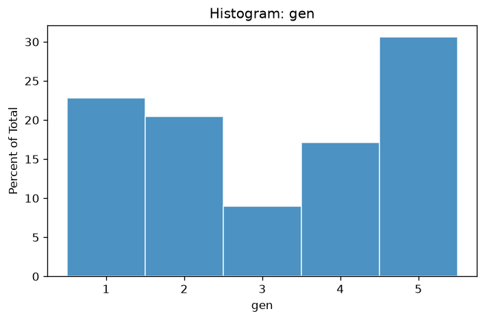
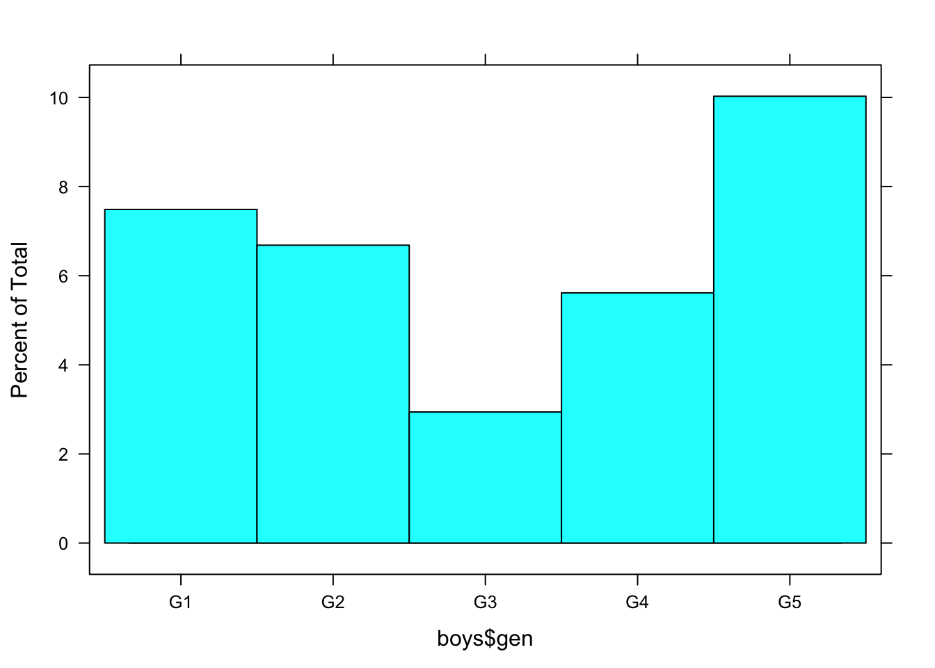
A histogram can be made with the function histogram().
Note: Matplotlib equivalent of the R lattice plot.
plot_histogram(boys, boy_names, 'gen')(plot below)histogram(boys$gen)plot_histogram(boys, boy_names, 'gen')(plot below)histogram(boys$gen)or, equivalently, one could use
histogram(~ gen, data = boys)
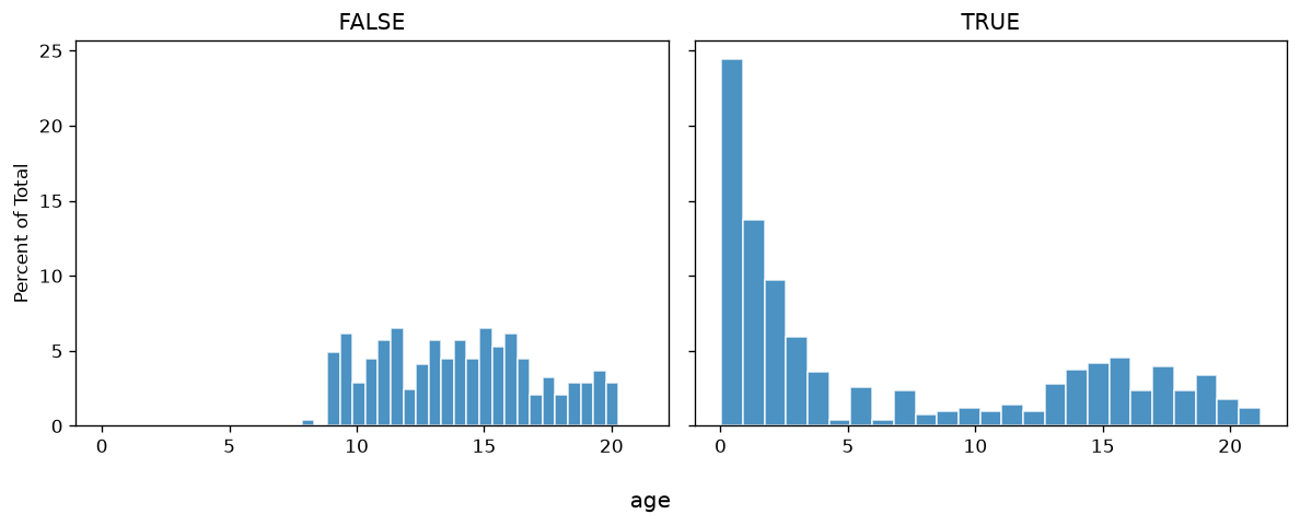
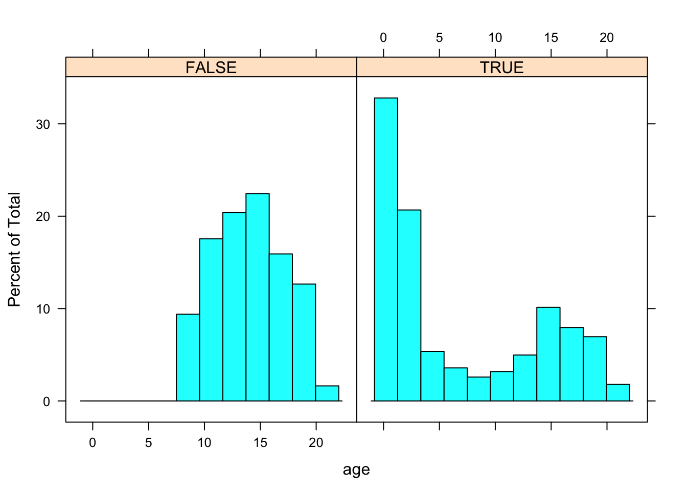
Writing the latter line of code for plots is more efficient than selecting every part of the boys data with the boys$... command, especially if plots become more advanced. The code for a conditional histogram of age given R is
Note: Matplotlib equivalent of the R lattice plot.
plot_histogram(boys, boy_names, 'age', condition=np.isnan(boys[:, gen_col]))(plot below)histogram(~age|R, data=boys)plot_histogram(boys, boy_names, 'age', condition=np.isnan(boys[:, gen_col]))(plot below)histogram(~age|R, data=boys)The histogram shows that the missingness in gen is not equally distributed across age.
7. Default MICE imputation
Note: Creates imp1 object; R vignette prints no console output here.
imp1 = mice(boys, column_names=boy_names, m=5, maxit=5, print_flag=False)(imputation complete — no printed output)imp1 <- mice(boys, print=FALSE)imp1 = mice(boys, column_names=boy_names, m=5, maxit=5, print_flag=False)(imputation complete — no printed output)imp1 <- mice(boys, print=FALSE)8. Compare imputed means
print(format_summary_boys_r(boys, boy_names)) age hgt wgt bmi
Min. : 0.035 Min. : 50.00 Min. : 3.14 Min. :11.77
1st Qu.: 1.581 1st Qu.: 84.88 1st Qu.: 11.70 1st Qu.:15.90
Median : 10.505 Median : 147.30 Median : 34.65 Median :17.45
Mean : 9.159 Mean : 132.15 Mean : 37.15 Mean :18.07
3rd Qu.: 15.267 3rd Qu.: 175.22 3rd Qu.: 59.58 3rd Qu.:19.53
Max. : 21.177 Max. : 198.00 Max. : 117.40 Max. :31.74
NA's :20 NA's : 4 NA's :21
hc gen phb tv reg
Min. :33.70 G1 : 56 P1 : 63 Min. : 1.00 north: 81
1st Qu.:48.12 G2 : 50 P2 : 40 1st Qu.: 4.00 east :161
Median :53.00 G3 : 22 P3 : 19 Median :12.00 west :239
Mean :51.51 G4 : 42 P4 : 32 Mean :11.89 south:191
3rd Qu.:56.00 G5 : 75 P5 : 50 3rd Qu.: 20.00 city : 73
Max. :65.00 NA's:503 P6 : 41 Max. :25.00 NA's : 3
NA's :46 NA's:503 NA's :522summary(boys) age hgt wgt bmi
Min. : 0.035 Min. : 50.00 Min. : 3.14 Min. :11.77
1st Qu.: 1.581 1st Qu.: 84.88 1st Qu.: 11.70 1st Qu.:15.90
Median :10.505 Median :147.30 Median : 34.65 Median :17.45
Mean : 9.159 Mean :132.15 Mean : 37.15 Mean :18.07
3rd Qu.:15.267 3rd Qu.:175.22 3rd Qu.: 59.58 3rd Qu.:19.53
Max. :21.177 Max. :198.00 Max. :117.40 Max. :31.74
NA's :20 NA's :4 NA's :21
hc gen phb tv reg
Min. :33.70 G1 : 56 P1 : 63 Min. : 1.00 north: 81
1st Qu.:48.12 G2 : 50 P2 : 40 1st Qu.: 4.00 east :161
Median :53.00 G3 : 22 P3 : 19 Median :12.00 west :239
Mean :51.51 G4 : 42 P4 : 32 Mean :11.89 south:191
3rd Qu.:56.00 G5 : 75 P5 : 50 3rd Qu.:20.00 city : 73
Max. :65.00 NA's:503 P6 : 41 Max. :25.00 NA's : 3
NA's :46 NA's:503 NA's :522print(format_summary_boys_r(boys, boy_names)) age hgt wgt bmi
Min. : 0.035 Min. : 50.00 Min. : 3.14 Min. :11.77
1st Qu.: 1.581 1st Qu.: 84.88 1st Qu.: 11.70 1st Qu.:15.90
Median : 10.505 Median : 147.30 Median : 34.65 Median :17.45
Mean : 9.159 Mean : 132.15 Mean : 37.15 Mean :18.07
3rd Qu.: 15.267 3rd Qu.: 175.22 3rd Qu.: 59.58 3rd Qu.:19.53
Max. : 21.177 Max. : 198.00 Max. : 117.40 Max. :31.74
NA's :20 NA's : 4 NA's :21
hc gen phb tv reg
Min. :33.70 G1 : 56 P1 : 63 Min. : 1.00 north: 81
1st Qu.:48.12 G2 : 50 P2 : 40 1st Qu.: 4.00 east :161
Median :53.00 G3 : 22 P3 : 19 Median :12.00 west :239
Mean :51.51 G4 : 42 P4 : 32 Mean :11.89 south:191
3rd Qu.:56.00 G5 : 75 P5 : 50 3rd Qu.: 20.00 city : 73
Max. :65.00 NA's:503 P6 : 41 Max. :25.00 NA's : 3
NA's :46 NA's:503 NA's :522summary(boys) age hgt wgt bmi
Min. : 0.035 Min. : 50.00 Min. : 3.14 Min. :11.77
1st Qu.: 1.581 1st Qu.: 84.88 1st Qu.: 11.70 1st Qu.:15.90
Median :10.505 Median :147.30 Median : 34.65 Median :17.45
Mean : 9.159 Mean :132.15 Mean : 37.15 Mean :18.07
3rd Qu.:15.267 3rd Qu.:175.22 3rd Qu.: 59.58 3rd Qu.:19.53
Max. :21.177 Max. :198.00 Max. :117.40 Max. :31.74
NA's :20 NA's :4 NA's :21
hc gen phb tv reg
Min. :33.70 G1 : 56 P1 : 63 Min. : 1.00 north: 81
1st Qu.:48.12 G2 : 50 P2 : 40 1st Qu.: 4.00 east :161
Median :53.00 G3 : 22 P3 : 19 Median :12.00 west :239
Mean :51.51 G4 : 42 P4 : 32 Mean :11.89 south:191
3rd Qu.:56.00 G5 : 75 P5 : 50 3rd Qu.:20.00 city : 73
Max. :65.00 NA's:503 P6 : 41 Max. :25.00 NA's : 3
NA's :46 NA's:503 NA's :522filled = complete(imp1, 1)
print(format_summary_boys_r(filled, boy_names, compact_factors=True))age hgt wgt bmi
Min. : 0.035 Min. : 50.00 Min. : 3.14 Min. :11.77
1st Qu.: 1.581 1st Qu.: 82.90 1st Qu.: 11.70 1st Qu.:15.89
Median : 10.505 Median : 145.75 Median : 34.55 Median :17.40
Mean : 9.159 Mean : 131.05 Mean : 37.15 Mean :18.04
3rd Qu.: 15.267 3rd Qu.: 175.00 3rd Qu.: 59.58 3rd Qu.:19.45
Max. : 21.177 Max. : 198.00 Max. : 117.40 Max. :31.74
hc gen phb tv reg
Min. :33.70 G1:384 P1:408 Min. : 1.000 north: 81
1st Qu.:48.45 G2: 87 P2: 56 1st Qu.: 2.000 east :162
Median :53.20 G3: 36 P3: 34 Median : 4.000 west :240
Mean :51.63 G4: 87 P4: 60 Mean : 8.389 south:191
3rd Qu.:56.00 G5:154 P5:106 3rd Qu.: 15.000 city : 74
Max. :65.00 P6: 84 Max. : 25.000summary(complete(imp1))age hgt wgt bmi
Min. : 0.035 Min. : 50.00 Min. : 3.14 Min. :11.77
1st Qu.: 1.581 1st Qu.: 82.90 1st Qu.: 11.70 1st Qu.:15.89
Median : 10.505 Median : 145.75 Median : 34.55 Median :17.40
Mean : 9.159 Mean : 131.05 Mean : 37.15 Mean :18.04
3rd Qu.: 15.267 3rd Qu.: 175.00 3rd Qu.: 59.58 3rd Qu.:19.45
Max. : 21.177 Max. : 198.00 Max. : 117.40 Max. :31.74
hc gen phb tv reg
Min. :33.70 G1:384 P1:408 Min. : 1.000 north: 81
1st Qu.:48.45 G2: 87 P2: 56 1st Qu.: 2.000 east :162
Median :53.20 G3: 36 P3: 34 Median : 4.000 west :240
Mean :51.63 G4: 87 P4: 60 Mean : 8.389 south:191
3rd Qu.:56.00 G5:154 P5:106 3rd Qu.: 15.000 city : 74
Max. :65.00 P6: 84 Max. : 25.000filled = complete(imp1, 1)
print(format_summary_boys_r(filled, boy_names, compact_factors=True))age hgt wgt bmi
Min. : 0.035 Min. : 50.00 Min. : 3.14 Min. :11.77
1st Qu.: 1.581 1st Qu.: 82.90 1st Qu.: 11.70 1st Qu.:15.89
Median : 10.505 Median : 145.75 Median : 34.55 Median :17.40
Mean : 9.159 Mean : 131.05 Mean : 37.15 Mean :18.04
3rd Qu.: 15.267 3rd Qu.: 175.00 3rd Qu.: 59.58 3rd Qu.:19.45
Max. : 21.177 Max. : 198.00 Max. : 117.40 Max. :31.74
hc gen phb tv reg
Min. :33.70 G1:384 P1:408 Min. : 1.000 north: 81
1st Qu.:48.45 G2: 87 P2: 56 1st Qu.: 2.000 east :162
Median :53.20 G3: 36 P3: 34 Median : 4.000 west :240
Mean :51.63 G4: 87 P4: 60 Mean : 8.389 south:191
3rd Qu.:56.00 G5:154 P5:106 3rd Qu.: 15.000 city : 74
Max. :65.00 P6: 84 Max. : 25.000summary(complete(imp1))age hgt wgt bmi
Min. : 0.035 Min. : 50.00 Min. : 3.14 Min. :11.77
1st Qu.: 1.581 1st Qu.: 82.90 1st Qu.: 11.70 1st Qu.:15.89
Median : 10.505 Median : 145.75 Median : 34.55 Median :17.40
Mean : 9.159 Mean : 131.05 Mean : 37.15 Mean :18.04
3rd Qu.: 15.267 3rd Qu.: 175.00 3rd Qu.: 59.58 3rd Qu.:19.45
Max. : 21.177 Max. : 198.00 Max. : 117.40 Max. :31.74
hc gen phb tv reg
Min. :33.70 G1:384 P1:408 Min. : 1.000 north: 81
1st Qu.:48.45 G2: 87 P2: 56 1st Qu.: 2.000 east :162
Median :53.20 G3: 36 P3: 34 Median : 4.000 west :240
Mean :51.63 G4: 87 P4: 60 Mean : 8.389 south:191
3rd Qu.:56.00 G5:154 P5:106 3rd Qu.: 15.000 city : 74
Max. :65.00 P6: 84 Max. : 25.000Most means are roughly equal, except the mean of tv, which is much lower in the first imputed data set, when compared to the incomplete data. This makes sense because most genital measures are unobserved for the lower ages. When imputing these values, the means should decrease.
Investigating univariate properties by using functions such as summary(), may not be ideal in the case of hundreds of variables. To extract just the information you need, for all imputed datasets, we can make use of the with() function. To obtain summaries for each imputed tv only, type
means = [np.nanmean(complete(imp1, i)[:, tv_idx]) for i in range(1, imp1.m + 1)]
print(format_tv_means_tibble_r(means))# A tibble: 5 x 1
x
<dbl>
1 8.39
2 8.50
3 8.42
4 8.48
5 8.47summary(with(imp1, mean(tv)))# A tibble: 5 x 1
x
<dbl>
1 8.39
2 8.50
3 8.42
4 8.48
5 8.47means = [np.nanmean(complete(imp1, i)[:, tv_idx]) for i in range(1, imp1.m + 1)]
print(format_tv_means_tibble_r(means))# A tibble: 5 x 1
x
<dbl>
1 8.39
2 8.50
3 8.42
4 8.48
5 8.47summary(with(imp1, mean(tv)))# A tibble: 5 x 1
x
<dbl>
1 8.39
2 8.50
3 8.42
4 8.48
5 8.47The importance of the imputation model
9. Inspect mammalsleep data
The mammalsleep dataset is part of mice. It contains the Allison and Cicchetti (1976) data for mammalian species. To learn more about this data, type
Note: Truncated R help excerpt (full pager is very long).
print(format_help_r('mammalsleep', max_lines=28))mammalsleep package:mice R Documentation
_M_a_m_m_a_l _s_l_e_e_p _d_a_t_a
_D_e_s_c_r_i_p_t_i_o_n:
Dataset from Allison and Cicchetti (1976) of 62 mammal species on
the interrelationship between sleep, ecological, and
constitutional variables. The dataset contains missing values on
five variables.
_F_o_r_m_a_t:
‘mammalsleep’ is a data frame with 62 rows and 11 columns:
species Species of animal
bw Body weight (kg)
brw Brain weight (g)
sws Slow wave ("nondreaming") sleep (hrs/day)
ps Paradoxical ("dreaming") sleep (hrs/day)
ts Total sleep (hrs/day) (sum of slow wave and paradoxical sleep)
mls Maximum life span (years)
... (33 more lines — full R help page omitted)help(mammalsleep)mammalsleep package:mice R Documentation
_M_a_m_m_a_l _s_l_e_e_p _d_a_t_a
_D_e_s_c_r_i_p_t_i_o_n:
Dataset from Allison and Cicchetti (1976) of 62 mammal species on
the interrelationship between sleep, ecological, and
constitutional variables. The dataset contains missing values on
five variables.
_F_o_r_m_a_t:
‘mammalsleep’ is a data frame with 62 rows and 11 columns:
species Species of animal
bw Body weight (kg)
brw Brain weight (g)
sws Slow wave ("nondreaming") sleep (hrs/day)
ps Paradoxical ("dreaming") sleep (hrs/day)
ts Total sleep (hrs/day) (sum of slow wave and paradoxical sleep)
mls Maximum life span (years)
gt Gestation time (days)
pi Predation index (1-5), 1 = least likely to be preyed upon
sei Sleep exposure index (1-5), 1 = least exposed (e.g. animal
sleeps in a well-protected den), 5 = most exposed
odi Overall danger index (1-5) based on the above two indices and
other information, 1 = least danger (from other animals), 5 =
most danger (from other animals)
_D_e_t_a_i_l_s:
Allison and Cicchetti (1976) investigated the interrelationship
between sleep, ecological, and constitutional variables. They
assessed these variables for 39 mammalian species. The authors
concluded that slow-wave sleep is negatively associated with a
factor related to body size. This suggests that large amounts of
this sleep phase are disadvantageous in large species. Also,
paradoxical sleep (REM sleep) was associated with a factor related
to predatory danger, suggesting that large amounts of this sleep
phase are disadvantageous in prey species.
_S_o_u_r_c_e:
Allison, T., Cicchetti, D.V. (1976). Sleep in Mammals: Ecological
and Constitutional Correlates. Science, 194(4266), 732-734.
_E_x_a_m_p_l_e_s:
sleep <- data(mammalsleep)print(format_help_r('mammalsleep', max_lines=28))mammalsleep package:mice R Documentation
_M_a_m_m_a_l _s_l_e_e_p _d_a_t_a
_D_e_s_c_r_i_p_t_i_o_n:
Dataset from Allison and Cicchetti (1976) of 62 mammal species on
the interrelationship between sleep, ecological, and
constitutional variables. The dataset contains missing values on
five variables.
_F_o_r_m_a_t:
‘mammalsleep’ is a data frame with 62 rows and 11 columns:
species Species of animal
bw Body weight (kg)
brw Brain weight (g)
sws Slow wave ("nondreaming") sleep (hrs/day)
ps Paradoxical ("dreaming") sleep (hrs/day)
ts Total sleep (hrs/day) (sum of slow wave and paradoxical sleep)
mls Maximum life span (years)
... (33 more lines — full R help page omitted)help(mammalsleep)mammalsleep package:mice R Documentation
_M_a_m_m_a_l _s_l_e_e_p _d_a_t_a
_D_e_s_c_r_i_p_t_i_o_n:
Dataset from Allison and Cicchetti (1976) of 62 mammal species on
the interrelationship between sleep, ecological, and
constitutional variables. The dataset contains missing values on
five variables.
_F_o_r_m_a_t:
‘mammalsleep’ is a data frame with 62 rows and 11 columns:
species Species of animal
bw Body weight (kg)
brw Brain weight (g)
sws Slow wave ("nondreaming") sleep (hrs/day)
ps Paradoxical ("dreaming") sleep (hrs/day)
ts Total sleep (hrs/day) (sum of slow wave and paradoxical sleep)
mls Maximum life span (years)
gt Gestation time (days)
pi Predation index (1-5), 1 = least likely to be preyed upon
sei Sleep exposure index (1-5), 1 = least exposed (e.g. animal
sleeps in a well-protected den), 5 = most exposed
odi Overall danger index (1-5) based on the above two indices and
other information, 1 = least danger (from other animals), 5 =
most danger (from other animals)
_D_e_t_a_i_l_s:
Allison and Cicchetti (1976) investigated the interrelationship
between sleep, ecological, and constitutional variables. They
assessed these variables for 39 mammalian species. The authors
concluded that slow-wave sleep is negatively associated with a
factor related to body size. This suggests that large amounts of
this sleep phase are disadvantageous in large species. Also,
paradoxical sleep (REM sleep) was associated with a factor related
to predatory danger, suggesting that large amounts of this sleep
phase are disadvantageous in prey species.
_S_o_u_r_c_e:
Allison, T., Cicchetti, D.V. (1976). Sleep in Mammals: Ecological
and Constitutional Correlates. Science, 194(4266), 732-734.
_E_x_a_m_p_l_e_s:
sleep <- data(mammalsleep)print(format_mammalsleep_head_r()) species bw brw sws ps ts mls gt pi sei
1 African elephant 6654.000 5712.0 NA NA 3.3 38.6 645 3 5
2 African giant pouched rat 1.000 6.6 6.3 2.0 8.3 4.5 42 3 1
3 Arctic Fox 3.385 44.5 NA NA 12.5 14.0 60 1 1
4 Arctic ground squirrel 0.920 5.7 NA NA 16.5 NA 25 5 2
5 Asian elephant 2547.000 4603.0 2.1 1.8 3.9 69.0 624 3 5
6 Baboon 10.550 179.5 9.1 0.7 9.8 27.0 180 4 4
odi
1 3
2 3
3 1
4 3
5 4
6 4head(mammalsleep) species bw brw sws ps ts mls gt pi sei
1 African elephant 6654.000 5712.0 NA NA 3.3 38.6 645 3 5
2 African giant pouched rat 1.000 6.6 6.3 2.0 8.3 4.5 42 3 1
3 Arctic Fox 3.385 44.5 NA NA 12.5 14.0 60 1 1
4 Arctic ground squirrel 0.920 5.7 NA NA 16.5 NA 25 5 2
5 Asian elephant 2547.000 4603.0 2.1 1.8 3.9 69.0 624 3 5
6 Baboon 10.550 179.5 9.1 0.7 9.8 27.0 180 4 4
odi
1 3
2 3
3 1
4 3
5 4
6 4print(format_mammalsleep_head_r()) species bw brw sws ps ts mls gt pi sei
1 African elephant 6654.000 5712.0 NA NA 3.3 38.6 645 3 5
2 African giant pouched rat 1.000 6.6 6.3 2.0 8.3 4.5 42 3 1
3 Arctic Fox 3.385 44.5 NA NA 12.5 14.0 60 1 1
4 Arctic ground squirrel 0.920 5.7 NA NA 16.5 NA 25 5 2
5 Asian elephant 2547.000 4603.0 2.1 1.8 3.9 69.0 624 3 5
6 Baboon 10.550 179.5 9.1 0.7 9.8 27.0 180 4 4
odi
1 3
2 3
3 1
4 3
5 4
6 4head(mammalsleep) species bw brw sws ps ts mls gt pi sei
1 African elephant 6654.000 5712.0 NA NA 3.3 38.6 645 3 5
2 African giant pouched rat 1.000 6.6 6.3 2.0 8.3 4.5 42 3 1
3 Arctic Fox 3.385 44.5 NA NA 12.5 14.0 60 1 1
4 Arctic ground squirrel 0.920 5.7 NA NA 16.5 NA 25 5 2
5 Asian elephant 2547.000 4603.0 2.1 1.8 3.9 69.0 624 3 5
6 Baboon 10.550 179.5 9.1 0.7 9.8 27.0 180 4 4
odi
1 3
2 3
3 1
4 3
5 4
6 4print(format_summary_mammalsleep_r(ms_full, ms_names)) species bw brw
African elephant : 1 Min. : 0.005 Min. : 0.14
African giant pouched rat: 1 1st Qu.: 0.600 1st Qu.: 4.25
Arctic Fox : 1 Median : 3.342 Median : 17.25
Arctic ground squirrel : 1 Mean : 198.790 Mean : 283.13
Asian elephant : 1 3rd Qu.: 48.203 3rd Qu.: 166.00
Baboon : 1 Max. :6654.000 Max. :5712.00
(Other) :56
sws ps ts mls
Min. : 2.100 Min. :0.000 Min. : 2.60 Min. : 2.000
1st Qu.: 6.250 1st Qu.:0.900 1st Qu.: 8.05 1st Qu.: 6.625
Median : 8.350 Median :1.800 Median :10.45 Median : 15.100
Mean : 8.673 Mean :1.972 Mean :10.53 Mean : 19.878
3rd Qu.: 11.000 3rd Qu.:2.550 3rd Qu.: 13.20 3rd Qu.: 27.750
Max. : 17.900 Max. :6.600 Max. : 19.90 Max. : 100.000
NA's :14 NA's :12 NA's : 4 NA's : 4
gt pi sei odi
Min. : 12.00 Min. : 1.000 Min. : 1.000 Min. : 1.000
1st Qu.: 35.75 1st Qu.: 2.000 1st Qu.: 1.000 1st Qu.: 1.000
Median : 79.00 Median : 3.000 Median : 2.000 Median : 2.000
Mean : 142.35 Mean : 2.871 Mean : 2.419 Mean : 2.613
3rd Qu.: 207.50 3rd Qu.: 4.000 3rd Qu.: 4.000 3rd Qu.: 4.000
Max. : 645.00 Max. : 5.000 Max. : 5.000 Max. : 5.000
NA's : 4summary(mammalsleep) species bw brw
African elephant : 1 Min. : 0.005 Min. : 0.14
African giant pouched rat: 1 1st Qu.: 0.600 1st Qu.: 4.25
Arctic Fox : 1 Median : 3.342 Median : 17.25
Arctic ground squirrel : 1 Mean : 198.790 Mean : 283.13
Asian elephant : 1 3rd Qu.: 48.203 3rd Qu.: 166.00
Baboon : 1 Max. :6654.000 Max. :5712.00
(Other) :56
sws ps ts mls
Min. : 2.100 Min. :0.000 Min. : 2.60 Min. : 2.000
1st Qu.: 6.250 1st Qu.:0.900 1st Qu.: 8.05 1st Qu.: 6.625
Median : 8.350 Median :1.800 Median :10.45 Median : 15.100
Mean : 8.673 Mean :1.972 Mean :10.53 Mean : 19.878
3rd Qu.:11.000 3rd Qu.:2.550 3rd Qu.:13.20 3rd Qu.: 27.750
Max. :17.900 Max. :6.600 Max. :19.90 Max. :100.000
NA's :14 NA's :12 NA's :4 NA's :4
gt pi sei odi
Min. : 12.00 Min. :1.000 Min. :1.000 Min. :1.000
1st Qu.: 35.75 1st Qu.:2.000 1st Qu.:1.000 1st Qu.:1.000
Median : 79.00 Median :3.000 Median :2.000 Median :2.000
Mean :142.35 Mean :2.871 Mean :2.419 Mean :2.613
3rd Qu.:207.50 3rd Qu.:4.000 3rd Qu.:4.000 3rd Qu.:4.000
Max. :645.00 Max. :5.000 Max. :5.000 Max. :5.000
NA's :4print(format_summary_mammalsleep_r(ms_full, ms_names)) species bw brw
African elephant : 1 Min. : 0.005 Min. : 0.14
African giant pouched rat: 1 1st Qu.: 0.600 1st Qu.: 4.25
Arctic Fox : 1 Median : 3.342 Median : 17.25
Arctic ground squirrel : 1 Mean : 198.790 Mean : 283.13
Asian elephant : 1 3rd Qu.: 48.203 3rd Qu.: 166.00
Baboon : 1 Max. :6654.000 Max. :5712.00
(Other) :56
sws ps ts mls
Min. : 2.100 Min. :0.000 Min. : 2.60 Min. : 2.000
1st Qu.: 6.250 1st Qu.:0.900 1st Qu.: 8.05 1st Qu.: 6.625
Median : 8.350 Median :1.800 Median :10.45 Median : 15.100
Mean : 8.673 Mean :1.972 Mean :10.53 Mean : 19.878
3rd Qu.: 11.000 3rd Qu.:2.550 3rd Qu.: 13.20 3rd Qu.: 27.750
Max. : 17.900 Max. :6.600 Max. : 19.90 Max. : 100.000
NA's :14 NA's :12 NA's : 4 NA's : 4
gt pi sei odi
Min. : 12.00 Min. : 1.000 Min. : 1.000 Min. : 1.000
1st Qu.: 35.75 1st Qu.: 2.000 1st Qu.: 1.000 1st Qu.: 1.000
Median : 79.00 Median : 3.000 Median : 2.000 Median : 2.000
Mean : 142.35 Mean : 2.871 Mean : 2.419 Mean : 2.613
3rd Qu.: 207.50 3rd Qu.: 4.000 3rd Qu.: 4.000 3rd Qu.: 4.000
Max. : 645.00 Max. : 5.000 Max. : 5.000 Max. : 5.000
NA's : 4summary(mammalsleep) species bw brw
African elephant : 1 Min. : 0.005 Min. : 0.14
African giant pouched rat: 1 1st Qu.: 0.600 1st Qu.: 4.25
Arctic Fox : 1 Median : 3.342 Median : 17.25
Arctic ground squirrel : 1 Mean : 198.790 Mean : 283.13
Asian elephant : 1 3rd Qu.: 48.203 3rd Qu.: 166.00
Baboon : 1 Max. :6654.000 Max. :5712.00
(Other) :56
sws ps ts mls
Min. : 2.100 Min. :0.000 Min. : 2.60 Min. : 2.000
1st Qu.: 6.250 1st Qu.:0.900 1st Qu.: 8.05 1st Qu.: 6.625
Median : 8.350 Median :1.800 Median :10.45 Median : 15.100
Mean : 8.673 Mean :1.972 Mean :10.53 Mean : 19.878
3rd Qu.:11.000 3rd Qu.:2.550 3rd Qu.:13.20 3rd Qu.: 27.750
Max. :17.900 Max. :6.600 Max. :19.90 Max. :100.000
NA's :14 NA's :12 NA's :4 NA's :4
gt pi sei odi
Min. : 12.00 Min. :1.000 Min. :1.000 Min. :1.000
1st Qu.: 35.75 1st Qu.:2.000 1st Qu.:1.000 1st Qu.:1.000
Median : 79.00 Median :3.000 Median :2.000 Median :2.000
Mean :142.35 Mean :2.871 Mean :2.419 Mean :2.613
3rd Qu.:207.50 3rd Qu.:4.000 3rd Qu.:4.000 3rd Qu.:4.000
Max. :645.00 Max. :5.000 Max. :5.000 Max. :5.000
NA's :4# str() layout — static R reference'data.frame': 62 obs. of 11 variables:
$ species: Factor w/ 62 levels "African elephant",..: 1 2 3 4 5 6 7 8 9 10 ...
$ bw : num 6654 1 3.38 0.92 2547 ...
$ brw : num 5712 6.6 44.5 5.7 4603 ...
$ sws : num NA 6.3 NA NA 2.1 9.1 15.8 5.2 10.9 8.3 ...
$ ps : num NA 2 NA NA 1.8 0.7 3.9 1 3.6 1.4 ...
$ ts : num 3.3 8.3 12.5 16.5 3.9 9.8 19.7 6.2 14.5 9.7 ...
$ mls : num 38.6 4.5 14 NA 69 27 19 30.4 28 50 ...
$ gt : num 645 42 60 25 624 180 35 392 63 230 ...
$ pi : int 3 3 1 5 3 4 1 4 1 1 ...
$ sei : int 5 1 1 2 5 4 1 5 2 1 ...
$ odi : int 3 3 1 3 4 4 1 4 1 1 ...str(mammalsleep)'data.frame': 62 obs. of 11 variables:
$ species: Factor w/ 62 levels "African elephant",..: 1 2 3 4 5 6 7 8 9 10 ...
$ bw : num 6654 1 3.38 0.92 2547 ...
$ brw : num 5712 6.6 44.5 5.7 4603 ...
$ sws : num NA 6.3 NA NA 2.1 9.1 15.8 5.2 10.9 8.3 ...
$ ps : num NA 2 NA NA 1.8 0.7 3.9 1 3.6 1.4 ...
$ ts : num 3.3 8.3 12.5 16.5 3.9 9.8 19.7 6.2 14.5 9.7 ...
$ mls : num 38.6 4.5 14 NA 69 27 19 30.4 28 50 ...
$ gt : num 645 42 60 25 624 180 35 392 63 230 ...
$ pi : int 3 3 1 5 3 4 1 4 1 1 ...
$ sei : int 5 1 1 2 5 4 1 5 2 1 ...
$ odi : int 3 3 1 3 4 4 1 4 1 1 ...# str() layout — static R reference'data.frame': 62 obs. of 11 variables:
$ species: Factor w/ 62 levels "African elephant",..: 1 2 3 4 5 6 7 8 9 10 ...
$ bw : num 6654 1 3.38 0.92 2547 ...
$ brw : num 5712 6.6 44.5 5.7 4603 ...
$ sws : num NA 6.3 NA NA 2.1 9.1 15.8 5.2 10.9 8.3 ...
$ ps : num NA 2 NA NA 1.8 0.7 3.9 1 3.6 1.4 ...
$ ts : num 3.3 8.3 12.5 16.5 3.9 9.8 19.7 6.2 14.5 9.7 ...
$ mls : num 38.6 4.5 14 NA 69 27 19 30.4 28 50 ...
$ gt : num 645 42 60 25 624 180 35 392 63 230 ...
$ pi : int 3 3 1 5 3 4 1 4 1 1 ...
$ sei : int 5 1 1 2 5 4 1 5 2 1 ...
$ odi : int 3 3 1 3 4 4 1 4 1 1 ...str(mammalsleep)'data.frame': 62 obs. of 11 variables:
$ species: Factor w/ 62 levels "African elephant",..: 1 2 3 4 5 6 7 8 9 10 ...
$ bw : num 6654 1 3.38 0.92 2547 ...
$ brw : num 5712 6.6 44.5 5.7 4603 ...
$ sws : num NA 6.3 NA NA 2.1 9.1 15.8 5.2 10.9 8.3 ...
$ ps : num NA 2 NA NA 1.8 0.7 3.9 1 3.6 1.4 ...
$ ts : num 3.3 8.3 12.5 16.5 3.9 9.8 19.7 6.2 14.5 9.7 ...
$ mls : num 38.6 4.5 14 NA 69 27 19 30.4 28 50 ...
$ gt : num 645 42 60 25 624 180 35 392 63 230 ...
$ pi : int 3 3 1 5 3 4 1 4 1 1 ...
$ sei : int 5 1 1 2 5 4 1 5 2 1 ...
$ odi : int 3 3 1 3 4 4 1 4 1 1 ...print(format_md_pattern_r(md_pattern(ms_full, ms_names))) species bw brw pi sei odi ts mls gt ps sws
42 1 1 1 1 1 1 1 1 1 1 1 0
9 1 1 1 1 1 1 1 1 1 0 0 2
3 1 1 1 1 1 1 1 1 0 1 1 1
2 1 1 1 1 1 1 1 0 1 1 1 1
1 1 1 1 1 1 1 1 0 1 0 0 3
1 1 1 1 1 1 1 1 0 0 1 1 2
2 1 1 1 1 1 1 0 1 1 1 0 2
2 1 1 1 1 1 1 0 1 1 0 0 3
0 0 0 0 0 0 4 4 4 12 14 38md.pattern(mammalsleep) species bw brw pi sei odi ts mls gt ps sws
42 1 1 1 1 1 1 1 1 1 1 1 0
9 1 1 1 1 1 1 1 1 1 0 0 2
3 1 1 1 1 1 1 1 1 0 1 1 1
2 1 1 1 1 1 1 1 0 1 1 1 1
1 1 1 1 1 1 1 1 0 1 0 0 3
1 1 1 1 1 1 1 1 0 0 1 1 2
2 1 1 1 1 1 1 0 1 1 1 0 2
2 1 1 1 1 1 1 0 1 1 0 0 3
0 0 0 0 0 0 4 4 4 12 14 38print(format_md_pattern_r(md_pattern(ms_full, ms_names))) species bw brw pi sei odi ts mls gt ps sws
42 1 1 1 1 1 1 1 1 1 1 1 0
9 1 1 1 1 1 1 1 1 1 0 0 2
3 1 1 1 1 1 1 1 1 0 1 1 1
2 1 1 1 1 1 1 1 0 1 1 1 1
1 1 1 1 1 1 1 1 0 1 0 0 3
1 1 1 1 1 1 1 1 0 0 1 1 2
2 1 1 1 1 1 1 0 1 1 1 0 2
2 1 1 1 1 1 1 0 1 1 0 0 3
0 0 0 0 0 0 4 4 4 12 14 38md.pattern(mammalsleep) species bw brw pi sei odi ts mls gt ps sws
42 1 1 1 1 1 1 1 1 1 1 1 0
9 1 1 1 1 1 1 1 1 1 0 0 2
3 1 1 1 1 1 1 1 1 0 1 1 1
2 1 1 1 1 1 1 1 0 1 1 1 1
1 1 1 1 1 1 1 1 0 1 0 0 3
1 1 1 1 1 1 1 1 0 0 1 1 2
2 1 1 1 1 1 1 0 1 1 1 0 2
2 1 1 1 1 1 1 0 1 1 0 0 3
0 0 0 0 0 0 4 4 4 12 14 38Answer: 8 patterns in total, with the pattern where everything is observed occuring the most (42 times).
10. Impute mammalsleep with PMM
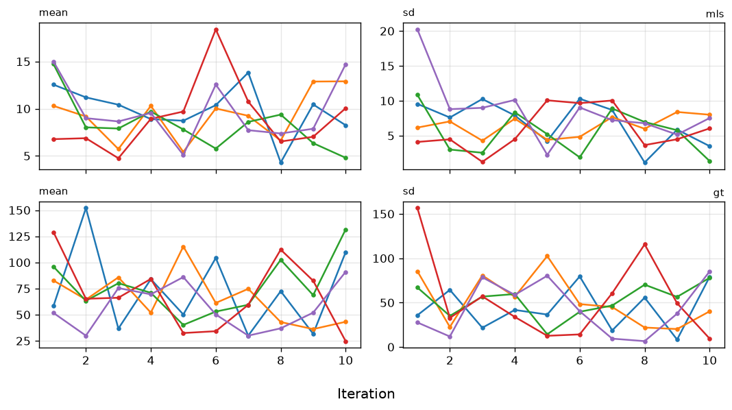
imp_ms = mice(ms_full, column_names=ms_names, m=5, maxit=10, print_flag=False)Warning: Number of logged events: 27imp <- mice(mammalsleep, maxit = 10, print=F)Warning: Number of logged events: 27imp_ms = mice(ms_full, column_names=ms_names, m=5, maxit=10, print_flag=False)Warning: Number of logged events: 27imp <- mice(mammalsleep, maxit = 10, print=F)Warning: Number of logged events: 27Inspect the trace lines
Note: Matplotlib equivalent of the R lattice plot.
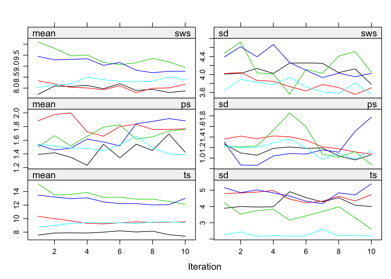
plot_mids(imp_ms, variables=['sws', 'ps', 'ts'])(plot below)plot(imp)plot_mids(imp_ms, variables=['sws', 'ps', 'ts'])(plot below)plot(imp)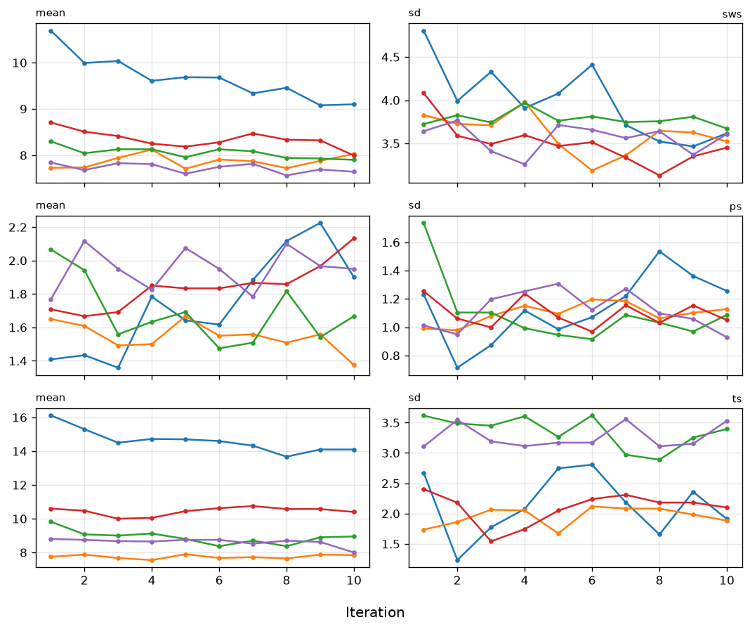
11. Regression on mammalsleep
fit1 = with_mids(imp_ms, formula='sws ~ log10(bw) + odi')(mira object created — no printed output)fit1 <- with(imp, lm(sws ~ log10(bw) + odi), print=F)fit1 = with_mids(imp_ms, formula='sws ~ log10(bw) + odi')(mira object created — no printed output)fit1 <- with(imp, lm(sws ~ log10(bw) + odi), print=F)12. Pool mammalsleep model
print(format_pool_mipo_r(pool(fit1)))Class: mipo m = 5
estimate ubar b t dfcom df
(Intercept) 11.3832377 0.59934692 0.03444354 0.6406792 59 50.60108
log10(bw) -1.1540768 0.08460947 0.00778340 0.0939495 59 45.62378
odi -0.8281281 0.07493542 0.00824923 0.0848345 59 43.04458
riv lambda fmi
(Intercept) 0.0689621 0.0645132 0.0994187
log10(bw) 0.1103904 0.0994159 0.1364588
odi 0.1321015 0.1166870 0.1550547pool(fit1)Class: mipo m = 5
estimate ubar b t dfcom df
(Intercept) 11.3832377 0.59934692 0.03444354 0.6406792 59 50.60108
log10(bw) -1.1540768 0.08460947 0.00778340 0.0939495 59 45.62378
odi -0.8281281 0.07493542 0.00824923 0.0848345 59 43.04458
riv lambda fmi
(Intercept) 0.0689621 0.0645132 0.0994187
log10(bw) 0.1103904 0.0994159 0.1364588
odi 0.1321015 0.1166870 0.1550547print(format_pool_mipo_r(pool(fit1)))Class: mipo m = 5
estimate ubar b t dfcom df
(Intercept) 11.3832377 0.59934692 0.03444354 0.6406792 59 50.60108
log10(bw) -1.1540768 0.08460947 0.00778340 0.0939495 59 45.62378
odi -0.8281281 0.07493542 0.00824923 0.0848345 59 43.04458
riv lambda fmi
(Intercept) 0.0689621 0.0645132 0.0994187
log10(bw) 0.1103904 0.0994159 0.1364588
odi 0.1321015 0.1166870 0.1550547pool(fit1)Class: mipo m = 5
estimate ubar b t dfcom df
(Intercept) 11.3832377 0.59934692 0.03444354 0.6406792 59 50.60108
log10(bw) -1.1540768 0.08460947 0.00778340 0.0939495 59 45.62378
odi -0.8281281 0.07493542 0.00824923 0.0848345 59 43.04458
riv lambda fmi
(Intercept) 0.0689621 0.0645132 0.0994187
log10(bw) 0.1103904 0.0994159 0.1364588
odi 0.1321015 0.1166870 0.1550547print(format_pool_v03_summary_r(summary_pool(pool(fit1)))) estimate std.error statistic df p.value
(Intercept) 11.3832377 0.8004244 14.221503 50.601082 0.000000000e+00
log10(bw) -1.1540768 0.3065119 -3.765194 45.623781 4.744272933e-04
odi -0.8281281 0.2912636 -2.843225 43.044582 6.804305093e-03summary(pool(fit1)) estimate std.error statistic df p.value
(Intercept) 11.3832377 0.8004244 14.221503 50.601082 0.000000000e+00
log10(bw) -1.1540768 0.3065119 -3.765194 45.623781 4.744272933e-04
odi -0.8281281 0.2912636 -2.843225 43.044582 6.804305093e-03print(format_pool_v03_summary_r(summary_pool(pool(fit1)))) estimate std.error statistic df p.value
(Intercept) 11.3832377 0.8004244 14.221503 50.601082 0.000000000e+00
log10(bw) -1.1540768 0.3065119 -3.765194 45.623781 4.744272933e-04
odi -0.8281281 0.2912636 -2.843225 43.044582 6.804305093e-03summary(pool(fit1)) estimate std.error statistic df p.value
(Intercept) 11.3832377 0.8004244 14.221503 50.601082 0.000000000e+00
log10(bw) -1.1540768 0.3065119 -3.765194 45.623781 4.744272933e-04
odi -0.8281281 0.2912636 -2.843225 43.044582 6.804305093e-03The fmi and lambda are much too high. This is due to species being included in the imputation model. Because there are 62 species and mice automatically converts factors (categorical variables) to dummy variables, each species is modeled by its own imputation model.
13. Drop species column
impnew = mice(ms_no_sp, column_names=ms_no_names, m=5, maxit=10, print_flag=False)Warning: Number of logged events: 15impnew <- mice(mammalsleep[ , -1], maxit = 10, print = F)Warning: Number of logged events: 15impnew = mice(ms_no_sp, column_names=ms_no_names, m=5, maxit=10, print_flag=False)Warning: Number of logged events: 15impnew <- mice(mammalsleep[ , -1], maxit = 10, print = F)Warning: Number of logged events: 1514. Re-impute without species
fit2 = with_mids(impnew, formula='sws ~ log10(bw) + odi')
print(format_pool_mipo_r(pool(fit2)))Class: mipo m = 5
estimate ubar b t dfcom df
(Intercept) 11.3500427 0.61817617 0.04037797 0.6666297 59 49.48618
log10(bw) -1.1079037 0.08726759 0.00546546 0.0938261 59 49.87051
odi -0.8082814 0.07728961 0.00810531 0.0870160 59 43.77962
riv lambda fmi
(Intercept) 0.0783815 0.0726844 0.1080200
log10(bw) 0.0751545 0.0699011 0.1050852
odi 0.1258433 0.1117769 0.1497517fit2 <- with(impnew, lm(sws ~ log10(bw) + odi))
pool(fit2)Class: mipo m = 5
estimate ubar b t dfcom df
(Intercept) 11.3500427 0.61817617 0.04037797 0.6666297 59 49.48618
log10(bw) -1.1079037 0.08726759 0.00546546 0.0938261 59 49.87051
odi -0.8082814 0.07728961 0.00810531 0.0870160 59 43.77962
riv lambda fmi
(Intercept) 0.0783815 0.0726844 0.1080200
log10(bw) 0.0751545 0.0699011 0.1050852
odi 0.1258433 0.1117769 0.1497517fit2 = with_mids(impnew, formula='sws ~ log10(bw) + odi')
print(format_pool_mipo_r(pool(fit2)))Class: mipo m = 5
estimate ubar b t dfcom df
(Intercept) 11.3500427 0.61817617 0.04037797 0.6666297 59 49.48618
log10(bw) -1.1079037 0.08726759 0.00546546 0.0938261 59 49.87051
odi -0.8082814 0.07728961 0.00810531 0.0870160 59 43.77962
riv lambda fmi
(Intercept) 0.0783815 0.0726844 0.1080200
log10(bw) 0.0751545 0.0699011 0.1050852
odi 0.1258433 0.1117769 0.1497517fit2 <- with(impnew, lm(sws ~ log10(bw) + odi))
pool(fit2)Class: mipo m = 5
estimate ubar b t dfcom df
(Intercept) 11.3500427 0.61817617 0.04037797 0.6666297 59 49.48618
log10(bw) -1.1079037 0.08726759 0.00546546 0.0938261 59 49.87051
odi -0.8082814 0.07728961 0.00810531 0.0870160 59 43.77962
riv lambda fmi
(Intercept) 0.0783815 0.0726844 0.1080200
log10(bw) 0.0751545 0.0699011 0.1050852
odi 0.1258433 0.1117769 0.1497517print(format_pool_v03_summary_r(summary_pool(pool(fit2)))) estimate std.error statistic df p.value
(Intercept) 11.3500427 0.8164740 13.901292 49.486180 0.000000000e+00
log10(bw) -1.1079037 0.3063105 -3.616930 49.870508 6.945071261e-04
odi -0.8082814 0.2949847 -2.740079 43.779621 8.854862806e-03summary(pool(fit2)) estimate std.error statistic df p.value
(Intercept) 11.3500427 0.8164740 13.901292 49.486180 0.000000000e+00
log10(bw) -1.1079037 0.3063105 -3.616930 49.870508 6.945071261e-04
odi -0.8082814 0.2949847 -2.740079 43.779621 8.854862806e-03print(format_pool_v03_summary_r(summary_pool(pool(fit2)))) estimate std.error statistic df p.value
(Intercept) 11.3500427 0.8164740 13.901292 49.486180 0.000000000e+00
log10(bw) -1.1079037 0.3063105 -3.616930 49.870508 6.945071261e-04
odi -0.8082814 0.2949847 -2.740079 43.779621 8.854862806e-03summary(pool(fit2)) estimate std.error statistic df p.value
(Intercept) 11.3500427 0.8164740 13.901292 49.486180 0.000000000e+00
log10(bw) -1.1079037 0.3063105 -3.616930 49.870508 6.945071261e-04
odi -0.8082814 0.2949847 -2.740079 43.779621 8.854862806e-03Note that the fmi and lambda have dramatically decreased. The imputation model has been greatly improved.
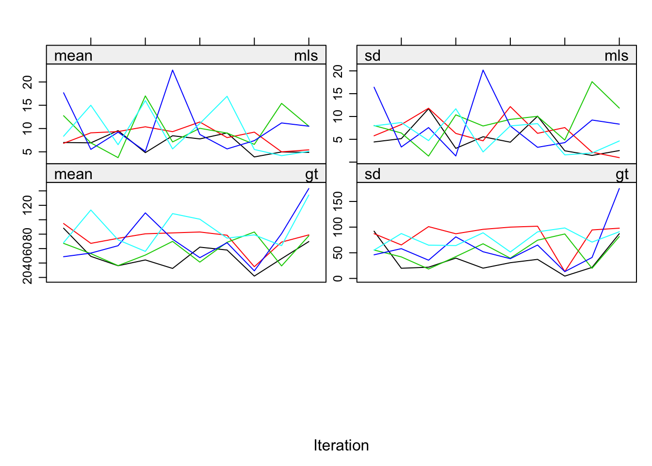
15. Trace plot for impnew
Note: Matplotlib equivalent of the R lattice plot.
plot_mids(impnew, variables=['mls', 'gt'])(plot below)plot(impnew)plot_mids(impnew, variables=['mls', 'gt'])(plot below)plot(impnew)Even though the fraction of information missing due to nonresponse (fmi) and the relative increase in variance due to nonresponse (lambda) are nice and low, the convergence turns out to be a real problem. The reason is the structure in the data. Total sleep (ts) is the sum of paradoxical sleep (ps) and short wave sleep (sws). This relation is ignored in the imputations, but it is necessary to take this relation into account. mice offers a routine called passive imputation, which allows users to take transformations, combinations and recoded variables into account when imputing their data.
We explain passive imputation in detail in the this vignette.
We have seen that the practical execution of multiple imputation and pooling is straightforward with the R package mice. The package is designed to allow you to assess and control the imputations themselves, the convergence of the algorithm and the distributions and multivariate relations of the observed and imputed data.
It is important to ‘gain’ this control as a user. After all, we are imputing values and we aim to properly adress the uncertainty about the missingness problem.
- End of Vignette